Filter

FIL bull-pollbakThe Filecoin ( BINANCE:FILUSDT ) chart, after a correction to $2.65, is attempting to pull back to the broken level around $2.77. If it fails to break this resistance, another decline towards support levels at $2.525 and then $2.39 is likely, which could act as a potential starting point for a new upward movement towards targets at $3.02 and $3.30.
🔑 Key Zones on the FIL Chart:
Primary Resistance: $2.77 (Pullback to broken level)
First Support: $2.525
Second Support: $2.39
First Bullish Target: $3.02
Second Bullish Target: $3.30

#FIL/USDT#FIL
The price is moving within a descending channel on the 1-hour frame, adhering well to it, and is heading towards a strong breakout and retest.
We are seeing a bounce from the lower boundary of the descending channel, which is support at 2.68.
We have a downtrend on the RSI indicator that is about to be broken and retested, which supports the upward trend.
We are looking for stability above the 100 moving average.
Entry price: 2.73
First target: 2.78
Second target: 2.86
Third target: 2.95

FIL short-down FILUSDT Signal
🔹 Key Resistance Level: $3.35 – $3.50
🔹 Important Support Levels: $3.148 – $2.940 – $2.738
Analysis:
FIL price has been moving in an uptrend within a rising wedge pattern and has now reached the key resistance zone of $3.35 – $3.50. If this level is broken, followed by confirmation with a pullback, the uptrend is likely to continue. However, failure to break this resistance could lead to a price correction toward the mentioned support levels.
📌 Trading Strategy:
✅ Sell Entry after breaking the uptrend and confirming below $3.148
🎯 Targets: $2.940 – $2.738
🛑 Stop Loss: $3.30
⚠ Important Note: Risk management should not be ignored!

#FIL/USDT#FIL
The price is moving in a descending channel on the 1-hour frame and is expected to continue upwards
We have a trend to stabilize above the moving average 100 again
We have a descending trend on the RSI indicator that supports the rise by breaking it upwards
We have a support area at the lower limit of the channel at a price of 5.80
Entry price 6.02
First target 6.15
Second target 6.34
Third target 6.60

#FIL/USDT Ready to go higher#FIL
The price is moving in a descending channel on the 1-hour frame and sticking to it well
We have a bounce from the lower limit of the descending channel, this support is at 4.70
We have a downtrend on the RSI indicator that is about to be broken, which supports the rise
We have a trend to stabilize above the moving average 100
Entry price 4.87
First target 5.22
Second target 5.49
Third target 5.82

#FIL/USDT Ready to go higher#FIL
The price is moving in a descending channel on the 1-hour frame and sticking to it well
We have a bounce from the lower limit of the descending channel, this support is at 5.80
We have a downtrend on the RSI indicator that is about to be broken, which supports the rise
We have a trend to stabilize above the moving average 100
Entry price 6.81
First target 7.20
Second target 7.84
Third target 8.40

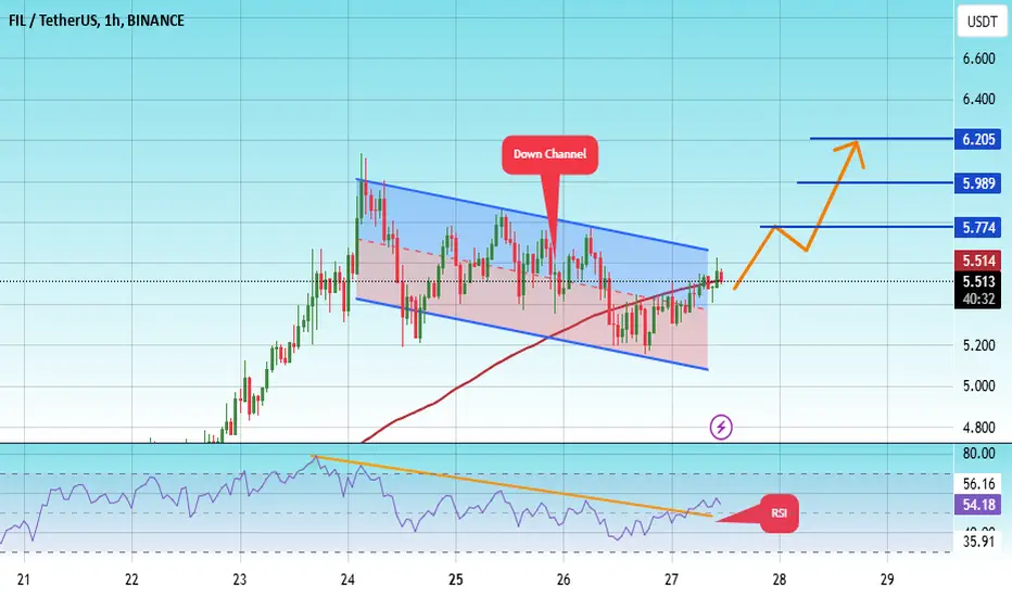
#FIL/USDT Ready to take off upwards#FIL
The price is moving in a descending channel on the 1-hour frame and sticking to it well
We have a bounce from the lower limit of the descending channel, this support is at 5.20
We have a downtrend on the RSI indicator that is about to break, which supports the rise
We have a trend to stabilize above the moving average 100
Entry price 5.50
First target 5.55
Second target 5.99
Third target 6.20
SNAP, YOU'RE NOT UGLY, YOU JUST NEED A FILTERSnapchat
talk about potential to target a very specific audience.
Teens
the AI potential is cool
I'm sure they will be going the reel route
Sell targets in Pink
Buy targets in blue
It seems this stock might have a little downside left, but should start going pretty soon.
somewhere between the blue range could easily trigger a really quick move to $20.
Earnings is the 23rd.
Really good looking chart for trading.
Watch the trends.

#FIL/USDT#FIL
The price is moving in a downward channel on a 4-hour frame, about to break upward
We have a Resin support area at $8
We have a downtrend on the RSI indicator about to occur. Bounce up
We have a higher stability moving average of 100
Entry price 9.14
First goal 10.07
The second goal is 10.70
Third goal 11.56

#FIL/USDT
#FIL
The price is moving in a triangle on the 4-hour frame and we have a green support area at $9
We have a higher stability of 100% moving forward
Now we have a nice breakout coming up
Our RSI indicator has a trend that is about to break to the upside
We are based on the rising trend
Entry price is 9.53
First goal 10.19
Second goal 11.12
For the target of the third 12.02

#FIL/USDT#FIL
The price has been moving in a downward channel since last April
The downtrend for that channel was broken at $3
It is the same strong support area
The price has gained nearly 200% so far
Supported by oversold on MACD
It is supported by the moving average 100 break of 1 D Frame
Current price 5.5 $
First goal 7.06 $
Second goal 9.11 $
The market's upward momentum will lead us to the expected targets
But be aware that there are some corrections

$BTC - Weekly Volatility flattening It looks like the volatility lines are flattening - To me there is a very good probability that we will come retest the $35k area sooner or later. If we don't go past this resistance level, thing will get bloody.

eurusd trading plan I expect that the price will retrace at Fibonaci 0.618 which is at 1.135 this is supported by a good drop base drop area I recommend buying for the short term and selling for the long term

RSI AMPLIFIER// (v4) RSI AMPLIFIER ( MCDX-Oscillator + Renko-Filter ) ( BTC ) ( 1h,2h,3h,4h )
//Authors credit:
//Smart Money based of / Indicator | MCDX
//Renko Volume based of "Weiss Wave Volume" / "WWV"
//The SmartMoney MCDX (MultiColor-Dragon) amplify rsi values to give confirmation of so called BANKER or SMART-MONEY against Retaillers.
//The main issue to me was that the original "SmartMoney MCDX" give only half the potential information since it focus only on positive price action.
//Therefore this version is a SMART-MONEY OSCILLATOR built to give entry/exit signals for shorts as well as long.
//The Real-Momentum plot replaces HOT MONEY (area, darkgreen/darkred), react quickly to oversold/overbought and hit the max/min value at almost every bar.
//The Over-Extended plot replaces BANKER MONEY (stepline, yellow/blue), need a stronger oversold/overbought value to move from the middle.
//The Signal-Line plot (line, green/red, with filler), is halfway between the Real-Mommentum & Over-Extended trying to give a signal after the move start but before the biggest candles.
//
//The original RETAILLERS MONEY carries no information and as been erased.
//
//Renko-Filter reduce the noise by adding volume values to each new columns until the trend reversal.
//How to use:
//
//The purpose and logic of this indicator is " Amplify to Simplify "
//
//Enter trade when the Signal-Line leave the middle.
//Long when it go TOP GREEN / Short when it go BOTTOM RED
//Exit trade when the Signal-Line return to middle or/while the Renko-Filter reverse.
//
//When you analyze the chart stay zoom out with max/min on the edges of the pan. Only the biggest Renko-series will be visible.
//When trading, you may zoom in to see evolution in real time.(version built for minutes time-frames in progress)
//
//You can easily set a LONG TRADE alarm on the Signal-Line, choosing "Greater than 10" then "Less than 50000"
//You can easily set a SHORT TRADE alarm on the Signal-Line, choosing "Less than -10" then "Greater than -50000"
//
//Be careful when Real-Momentum start being choppy or simply goes too much/too long in the opposite side of the trend.
//If the Over-Extended plot follow the Signal-Line after you enter a trade, you're good but always exit before the Over-Extended return to mid.
//Use the Renko-Filter to detect lauching Extended-Trend, to confirm Real-Momentum reversal, or to stay in a trade to the last candles.
// INFO:
//This version is built on purpose for BTC 1h/2h/3h/4h, differents assets, time-frames or exchanges may need change.
//If you can't see the Over-Extended, Signal Line or Renko-Filter with a particular time-frame or asset, you can change the value of the rsi at "rsi := 500000" & "rsi := -500000".
//Change by a value > to that of the candles (last value in status line).
//Zoom in on the indicator to see the Renko-Filter but idealy you want to see the max/min value of the 3 plot of the indicator(default = 50000).
//
// Overlay:
//You can display this indicator directly on your Chart and set No scale (fullscreen), to use it like as a RSI Baseline.
//If so, i made specifics version doing it by default (overlay,BTC)(overlay,largeCAP).
//@version=4

Make Indicators Profitable AgainIf you have been in the market for some time, then you have probably tried a few different indicators. Some may have worked well, others not so much. However, just because the indicator's default version didn't work, that doesn't mean it doesn't have potential!
Parabolic SAR Default
We have tested the Parabolic SAR with its default settings, on ETH/USDT 4h chart, on Kucoin. Each trade was taken with 100% of the available equity, and resulted in a total profit of -89%. This means that you would have decimated your account if you had used the default Parabolic SAR. The default Parabolic SAR values on Tradingview are: "Start" 0.02, "Increment" 0.02 and "Maximum" 0.2.
Modified Parabolic SAR
By modifying the "Increment" and "Maximum" values to 0.002, you will create a version that has a total profit of 492%! This version even works on shorts. There are even more profitable versions of the Parabolic SAR strategies which you can use. We have just tested a few different values, but more extensive testing would almost certainly bring better results.
Although you can use this indicator for your entries and exits, it is better to use it as a filter. This version is a lot slower than the default one, and as such, it only catches the big trends. As mentioned earlier, it also works on shorts; therefore, it can identify bear markets accurately. Therefore, you can use this version as a filter to find the long-term trend, and then use another indicator that signals more often, such as the MACD, to find the appropriate entries and exits.

GBPCAD Sell Setup!Hello everyone, if you like the idea, do not forget to support with a like and follow.
on DAILY: GBPCAD is sitting around a strong resistance/supply in blue so we will be looking for sell setups on lower timeframes.
on H1: GBPCAD formed a valid trendline in red.
Trigger: Waiting for a momentum candle close below the gray area / neckline to sell.
NB: Until the sell is activated, this one would be overall bullish .
Good luck!

Why A Cascading SMA Approximate A Gaussian Filter ?Introduction
The gaussian filter don't see many uses in technical analysis and financial data smoothing in general, however it possess really interesting properties and a really close relationship with the simple moving average.
The gaussian filter is a filter which possess a function approximately gaussian (bell shaped curve) as : impulse response, step response and frequency response. This characteristic is pretty cool actually, the gaussian function is always mysterious.
Now why do I talk about sma and estimation ? Well it is true, you can estimate a gaussian filter by applying an sma to another sma and so on such as : sma(...sma())
But why ? Just why is that so ? Well there are a lot of explanations, some of them involving the central limit theorem which would lead to a statistical explanation but I'll give a simpler explanation of this case by using signal processing.
Understanding Impulses Responses
The impulse response of a filter is the filter output using an impulse function as input or more simply : filter(impulse)
The impulse function is a simple function equal to 1 at a certain point in time, for example we can use : impulse = 1 if t = 10 else 0, where t = 1,2,3...inf
The impulse response of a filter tell us how to actually make the filter, for example :
a = filter(impulse)
b = sum(input*a) = filter(input)
This process is called convolution, and is simply the sum of the product of two functions, the input function and the kernel function, a kernel is just a way to say filter coefficients.
The Explanation
Now that you know that, let's explain why sma(...sma()) approximate a gaussian filter.
To do so let's take an impulse function and let's start applying an sma to it such as sma(impulse) (the sma period doesn't matter here)
Only one sma give a constant, let's use two sma's such as sma(sma(impulse))
This give us a triangular function, this is why sma(sma()) is often called triangular moving average, now let's repeat the process and add more sma's.
Do you see ? We are approximating a gaussian curve, if we do it many times the approximation will be even more correct.
Now let's recall :
The impulse response of a gaussian filter is a gaussian function f
The impulse response of many sma's give a function f' who approximate a gaussian function, therefore f ≈ f'
So sum(input*f') ≈ sum(input*f) and therefore sma(...sma(input)) ≈ gaussfilter(input)
Note : the process of applying a filter several time is called cascading
Conclusion
Simple isn't it ? The simple moving average is always fun to use and posses many properties, now you don't want to use such method because it's mega inefficient.
But maybe that you want to know about an efficient gaussian filter implementation ? I can work on it. Thanks for reading !

Today's Tutorial : How to filter good content in TradingViewHope this idea will inspire some of you !
Don't forget to hit the like/follow button if you feel like this post deserves it ;)
That's the best way to support me and help pushing this content to other users.
Kindly,
Phil

Digital Filters And DSPIntroduction
Digital signal processing (dsp) is used to manipulate signals and extract information from them. Among all the tools available, digital filters are the most common ones to use, in fact you are certainly using one during your analysis. In this post i will share some of the knowledge i have associated with filters and their properties.
I will try to be the more simple possible with my explanations for those with a light mathematical background :)
Before starting talking about filters, lets see some elementary things about dsp, this will help you understand what we will see next.
Time Domain
It is possible to see signals in different domains. The time domain show the signal with respect to time. For example when you see a price chart you see the price with respect to time, so you are on the time domain. A signal in the time domain is "one dimensional" because there is only one independent variables.
Frequency Domain
Frequency domain is another way to see a signal, this show the signal with respect to a frequency, in fact you are seeing the frequency content of the signal. In order to understand this i will introduce you to another powerful tool of digital signal processing, the "Fourier Transform". Lets look at some graphical explanations.
Lets take a signal we will call S
This signal is actually the sum of 3 Sine waves of different Frequencies
The one in red have a frequency of 0.07, the one in yellow have a frequency of 0.04 and the one in purple a frequency of 0.02, frequency is defined as the number of cycles in 1 unit time and is expressed in hertz Hz , here we will use "price bar" as unit time, it will be easier to see it this way. The Period is the reciprocal of the frequency, its the number of price bars in 1 cycle. To convert a frequency to a period just divide 1 by the frequency. The amplitude is the maximum absolute value of the signal, often said peak amplitude, for our sine waves the amplitude is 1.
So what does the Fourier transform ? Well the Fourier transform convert a signal in the time domain to the frequency domain. In other terms it decompose our signal in a sum of sine waves of different frequency and amplitude.In our signal S its Fourier transform would look like this :
Each bar is called a frequency bin or frequency component, they show the frequency and amplitude of one sine wave, each color represent the color of each sine waves i showed earlier. The abscissa x represent the frequency, the ordinate y represent the amplitude. Frequency bins on the left have a lower frequency than those in the right. If we sum each sine waves with the frequency and amplitude each bins give us we would get back our signal S
Its important to know this since filters interact with the frequency content, and the Fourier transform can tell us how.
What Is A Filter ?
A filter is processing tool that allow us to modify the frequency content of a signal, this mean that if we filter a signal, we will remove or change the amplitude of each frequency bin.
Interaction With The Frequency Domain
We will later see filters in the time domain but lets see them in frequency domain for the moment. In order to see how a filter interact with the frequency content of a signal we must look at the frequency response of the filter. A frequency response look like this :
The frequency response is shown in the frequency domain. So what does the red curve represent ? Well this curve show us how the filter interact with each frequency component, lets look at some terms of the frequency response.
The pass band area let each frequency components in that area unchanged, the stop band attenuation or transition band area only change the amplitude of each frequency components in that area, the stop band area remove each frequency components in that area. For example :
Here we have the frequency domain of a signal, after passing a filter to this signal the frequency domain will look like this :
In the image showed earlier you have a blue line, this line delimit the boundary between the pass band and the stop band attenuation, and this boundary is named cutoff frequency , the cutoff frequency is a value expressed in hertz. Actually when you are using a moving average, the length parameter control the position of the cutoff, but we will see moving averages later in more depth.
Types Of Filters
Now that we understand how a filter interact with frequency domain we must talk about different types of filters, filters can interact in different ways with the frequency components.
Low Pass Filters :
The name is straightforward, those filters let pass low frequency components and remove the high ones. Frequency response of low pass filters look like this :
High Pass Filters :
They let pass high frequency components while removing low ones.
Bandpass Filters :
A mix of the two previous filters, they let pass frequency components in a certain range.
Those can have two-cutoff f1, f2 with bandwidth f2 - f1 or one cutoff and one bandwidth parameter.
Band-Stop Filters :
Sometime called Notch filters or band-reject, they do the contrary of the bandpass filter, instead of letting pass frequency components in a certain range they remove them.
Design Of Different Types Of Filters
Low Pass Filters :
Low pass filters are used to remove high frequencies, when you remove high frequency components of a signal the result is a smoother signal, high frequency create irregularities in a signal and create roughness this is why the result is smoother. Low pass filters are also the core of the design of other filter types. The simplest low pass filter is called a simple moving average or running/rolling - mean/average, or boxcar filter, you will understand why the name "Boxcar" later.
The average value or mean of a signal is the sum of all values divided by the number of values, a moving average instead of using all the values will use a proportion of them.A simple moving average can be computed in different ways, here are the easiest ones.
1/n * sum(S,n)
sum(1/n * S,n)
sum(S,n)/n
change(cum(S),n)/n
where S is the signal we want to filter and n the period or number of data points we want to average.
The frequency response of a simple moving average look like this :
The higher the period the more little bumps in the stop band will be created, this is why the moving average still appear a bit rough, its because not all the frequencies in the stop band are removed, some are just attenuated. Those "bumps" are called ripples, when they are situated in the pass band we call them pass band ripples, when they are in the stop band we call them stop band ripples. We will later see filters who does not have ripples.
High Pass Filters
They remove low frequencies of a signal, its really easy to calculate those, the only thing you have to do is subtract your signal S with a low pass filter, the result show all the signal who have been filtered by the low pass filters. The frequency response of the low pass filter is then reversed. Here the frequency response of a high pass moving average filter :
They are really useful because its quite hard to forecast trends in a signal, but its way easier to forecast mid term cycles.
Bandpass Filters
They let pass frequencies in a range and they are also really easy to compute, first compute a high-pass filter by subtracting the price to a moving average low pass filter, then apply a low pass filter to the result and you end up with a bandpass filter, easy isn't it ? When creating a bandpass filter you can get the pictures of the frequency response of the filter during each step.
First step -> high pass filtering
Second Step -> Low pass filtering of the first step result
Band-Stop Filter
They are the opposite of the bandpass filter, so in order to construct those you just need you signal S and your signal S filtered by a bandpass filter. Subtract your signal S with the bandpass filtered version and you get a band-stop filter.
Filter Lag
Lag is defined as the effect of filters to show past frequencies, this delay is quite unfortunate for us since a filter with zero lag would violate causality and could provide what is called "The Holy Grail". However it is possible to minimize lag, one way is to amplify a frequency range of the signal and then filter the result, a filter describing this process is the zero-lag exponential moving average in the form of :
L = (Period - 1)/2
Y0 = S + (S - S(L)) -> Amplification Process
Y1 = EMA(Y0,Period) -> Filtering Process
Other methods exist but at the end getting optimal smoothing with minimum lag is not something classical filters can do. This is why adaptive filters such as Kalman and Wiener filters where made, but this is another subject that is more complicated.
Impulse Response
We are entering a really interesting topic, the topic of impulses responses and convolution. First what is an impulse ? An impulse is just defined as a really brief signal, here an example
The impulse response denoted h(t) is the reaction of a system to an impulse, so the impulse response of a filter is the filter using an impulse an input. Now lets see the impulse response of a simple moving average of period 5 (n = 5) , you will understand why they are called boxcar filters.
its just a "box", puns apart there is also something more than incredible with impulse responses, do you remember how to construct a moving average ? One of the ways was : sum(1/n * S,n) , 1/5 = 0.2, now look at the impulse response from closer
Its 0.2, or 1/5, nice isn't it ? When the impulse is equal to 1, the impulse response of a filter h(t) give us values called filter coefficients and this introduce the concept of convolution.
Convolution
The subject is vast but in resume convolution is the process of combining two function to create a third function. The symbol of convolution is ∗ not to be confounded with * who is used for multiplication.
To make it easier to understand convolution lets take back our 5 period moving average case and its impulse response h(t) . Now lets make an operation describing convolution
S ∗ h(t) = sum(S * h(t),5)
This operation give us a moving average of period 5. So impulse responses can give you really useful information about your filter.
IIR Filters
There are 2 filter family, F inite I mpulse R esponse filters or FIR and I nfinite I mpulse R esponse filters. IIR filters use recursion, this mean that they use output values as input, if we check the impulse response of those filter h(t) you will see that h(t) goes on forever after the impulse, this is why they are called infinite impulse response. The most well known IIR filter is the exponential moving average (ema), or exponential averager which is described as :
y = aS(t) + (1-a)y(t-1)
where a is called a smoothing constant and 0 < a < 1 .
An IIR filter can also be in the more common form :
y(t) = a0 * S(t) + a1 * S(t-1) + b1 * y(t-1)
Advanced Filter Design
Based on which filter you want to design (FIR/IIR) you will use different methods. FIR filters are easier to design, first select what frequency response your filter should have, then compute the Fourier transform of this frequency response, this will give you the impulse response and therefore the coefficients of the filter you want to design, then you only need to apply convolution. So basically, the Fourier transform of the filter impulse response give you the frequency response of the filter and vice versa.
IIR filters are way more complicated to design, you will need the z-transform and this is something that i don't really know about, how unfortunate.
Conclusions
I hope it wasn't that complicated because it shouldn't be, of course you can make filters without knowing all this, but its always cool to have more information. If you don't understand something or think i have made an error somewhere don't hesitate to mention it in the comment :)
Thanks for reading !

Improve your trading strategy with a trend filterWatch this video to learn about how you can improve and supplement your trading strategy with a trend filter.

The Moving Average Crossover Strategy - How to choose the best?Hey there!
Well, this is not a trading idea actually. I just want to present my new tool to the community.
This tool will help you to choose a type of moving average to create the most profitable trading system based on crossovers.
Click on the price scale, point to "Labels" and switch off "No Overlapping Labels" option to get a better view.
Detailed description can be found here .
I repeat
NOTE: The results may vary on different tickers and timeframes.
If you see the preview result it doesn't mean that these crossovers will be profitable on other instruments and timeframes. This is a normal situation because time series and their characteristics differ.
I know that because I tested this tool before publishing.
NOTE 2: You can use this tool by yourself and experiment with it, or you can order a study and I will share the spreadsheet that contains results. PM me for more details.
Good luck and happy trading!

Fibo support holding for $BTC.. staying long for nowNo break yet.. yes traded through, but I like to filter possible breaks
Need 3 consecutive days settle underneath the
61.8% level (only 1 happened)
or
a close 3% or more under the 61.8% level
(nope)
staying long for now!
Thoughts?
