VKM-RangeTrap-Indicator v1.1VKM-RangeTrap-Indicator v1.1 (AUDCAD M5)
Indicator Name: VKM-RangeTrap-Indicator v1.1
Recommended Timeframe: M5
Example Pair: AUDCAD
Method: VWAP-based range-reversal trading
🧭 Strategy Concept
AUDCAD is known for its narrow daily range and frequent sideways movements, especially during the Asian and early European sessions.
The VKM-RangeTrap strategy takes advantage of this characteristic by using VWAP (Volume Weighted Average Price) and its standard-deviation envelopes (Sigma) to detect temporary overbought and oversold zones.
When the price touches or breaks below the lower VWAP-Sigma band, it indicates a temporary oversold area → BUY signal.
When the price touches or breaks above the upper VWAP-Sigma band, it shows temporary overbought conditions → SELL signal.
A CCI(20) filter can be used to confirm momentum reversal (signals trigger only when CCI crosses the zero line).
⚙️ Basic Configuration
Range Method: VWAP
Sigma (Standard Deviation): 5
Sigma Length: 20
Confirmation Filter: CCI(20)
Signals: Green arrow (BUY) and red arrow (SELL) plotted directly on the chart
💡 Suggested Trading Approach
Timeframe: M5 (M3 if you want denser signals)
Entry Rules:
BUY when a green arrow appears near the VWAP-Lower support zone.
SELL when a red arrow appears near the VWAP-Upper resistance zone.
Take Profit: Use R:R ≈ 1:1.5 or an ATR-based trailing stop.
Stop Loss: Beyond the corresponding VWAP boundary or 10–20 pips away depending on volatility.
Best Conditions: Ranging or balanced markets (Asian session or early London).
📈 Performance on AUDCAD M5
AUDCAD typically moves in a stable 20–40-pip range, making it ideal for VWAP range-based trading.
The indicator performs best in sideways or mild pullback phases within larger trends.
With the CCI filter enabled, false signals are greatly reduced, resulting in steady scalping opportunities.
Suitable for day traders and scalpers aiming to profit from frequent VWAP reversals throughout the day.
⚠️ Notes
This is a range-reversal indicator, not a trend-following system.
Avoid trading during high-volatility news releases when VWAP bands expand sharply.
Can be combined with momentum indicators (ADX, WaveTrend, etc.) for stronger confirmation.
Indicators and strategies


Valdex BBWP Multitimeframe🇬🇧 (English Version)
Valdex BBWP Multitimeframe: Multitimeframe Volatility.
**Created by:**
**Adaptation of: Bollinger Band Width Percentile (BBWP)
📄 General Description
The **Valdex BBWP Multitimeframe** indicator is an advanced and optimized adaptation of the classic *Bollinger Band Width Percentile (BBWP)* indicator. Its purpose is to provide a robust and flexible tool for measuring the market's **relative volatility** on a scale from 0 to 100.
What distinguishes this version is its ability to **analyze volatility across THREE timeframes simultaneously**, allowing you to confirm expansion (high volatility) or contraction (low volatility) in higher timeframes without switching charts. It is an essential filter for any breakout or retracement strategy.
✨ Key Features
The indicator plots three volatility lines, each with a specific and independently configurable purpose:
1. **Base Line (Current TF):** Displays the BBWP calculated on the **exact timeframe of the current chart**, preserving its pure, unsmoothed value (original "noise").
2. **Multitimeframe (MTF) Lines:** Allows you to define two completely separate BBWP lines, each pulling data from an **external timeframe** (e.g., 60 minutes, Daily). Includes a **configurable Moving Average (MA)** to smooth the noise.
⚙️ Configuration and Usage
* **BBWP Base Settings:** You can configure the underlying BBWP parameters: Bands Length (13 default) and Percentile Lookback (252 default).
* **MTF Configuration:** For Lines 2 and 3, you **must manually enter** the desired timeframe in the text field (valid examples: `5`, `60`, `240`, `D`, `W`).

Lot Size CalculatorLot Size Calculator for Gold (XAU)
This indicator helps traders calculate the proper lot size for Gold (XAU) based on their entry, stop loss, and risk amount in USD.
You can set your entry and stop levels directly on the chart, and adjust your dollar risk from the settings panel.
The indicator measures the distance between entry and stop to calculate the position size that matches your selected risk.
A clean, customizable table displays key values such as Risk, Entry, Stop, Target, Lots, and Pips.
You can easily hide specific rows, change colors, and adjust layout options to fit your chart style.
Designed specifically for Gold traders, this tool provides a simple and visual way to manage risk directly on the chart.

Smarter Money Volume Rejection Blocks [PhenLabs]📊 Smarter Money Volume Rejection Blocks – Institutional Rejection Zone Detection
The Smarter Money Volume Rejection Blocks indicator combines high-volume analysis with statistical confidence intervals to identify where institutional traders are actively defending price levels through volume spikes and rejection patterns.
🔥 Core Methodology
Volume Spike Detection analyzes when current volume exceeds moving average by configurable multipliers (1.0-5.0x) to identify institutional activity
Rejection Candle Analysis uses dual-ratio system measuring wick percentage (30-90%) and maximum body ratio (10-60%) to confirm genuine rejections
Statistical Confidence Channels create three-level zones (upper, center, lower) based on ATR or Standard Deviation calculations
Smart Invalidation Logic automatically clears zones when price significantly breaches confidence levels to maintain relevance
Dynamic Channel Projection extends confidence intervals forward up to 200 bars with customizable length
Support Zone Identification detects bullish rejections where smart money absorbs selling pressure with high volume and strong lower wicks
Resistance Zone Mapping identifies bearish rejections where institutions defend price levels with volume spikes and pronounced upper wicks
Visual Information Dashboard displays real-time status table showing volume spike conditions and active support/resistance zones
⚙️ Technical Configuration
Dual Confidence Interval Methods: Choose between ATR-Based for trend-following environments or StdDev-Based for range-bound statistical precision
Volume Moving Average: Configurable period (default 20) for baseline volume comparison calculations
Volume Spike Multiplier: Adjustable threshold from 1.0 to 5.0 times average volume to filter institutional activity
Rejection Wick Percentage: Set minimum wick size from 30% to 90% of candle range for valid rejection detection
Maximum Body Ratio: Configure body-to-range ratio from 10% to 60% to ensure genuine rejection structures
Confidence Multiplier: Statistical multiplier (default 1.96) for 95% confidence interval calculations
Channel Projection Length: Extend confidence zones forward from 10 to 200 bars for anticipatory analysis
ATR Period: Customize Average True Range lookback from 5 to 50 bars for volatility-based calculations
StdDev Period: Adjust Standard Deviation period from 10 to 100 bars for statistical precision
🎯 Real-World Trading Applications
Identify high-probability support zones where institutional buyers have historically defended price with significant volume
Map resistance levels where smart money sellers consistently reject higher prices with volume confirmation
Combine with price action analysis to confirm breakout validity when price approaches confidence channel boundaries
Use invalidation signals to exit positions when smart money zones are definitively breached
Monitor the real-time dashboard to quickly assess current market structure and active rejection zones
Adapt strategy based on calculation method: ATR for trending markets, StdDev for ranging conditions
Set alerts on confidence level breaches to catch potential trend reversals or continuation patterns
📈 Visual Interpretation Guide
Green Zones indicate bullish rejection blocks where buyers defended with high volume and lower wicks
Red Zones indicate bearish rejection blocks where sellers defended with high volume and upper wicks
Solid Center Lines represent the core rejection price level where maximum volume activity occurred
Dashed Confidence Boundaries show upper and lower statistical limits based on volatility calculations
Zone Opacity decreases as channels extend forward to indicate decreasing confidence over time
Dashboard Color Coding provides instant visual feedback on active volume spike and zone conditions
⚠️ Important Considerations
Volume-based indicators identify historical rejection zones but cannot predict future price action with certainty
Market conditions change rapidly and institutional activity patterns evolve continuously
High volume does not guarantee level defense as market structure can shift without warning
Confidence intervals represent statistical probabilities, not guaranteed price boundaries

OsMA by A8/4 - Limited Edition🌟 **OsMA by A8/4 — The Ultimate Indicator for XAUUSD Trading** 🌟
An intelligent **automated system** designed exclusively for **gold trading**, equipped with everything you need in one tool 🔥
💡 **Key Features of OsMA by A8/4**
✅ **Auto Entry Signals**
Automatically detects trade opportunities using a **refined MACD Histogram formula** for enhanced accuracy.
Displays **LONG/SHORT arrows only on the first bar** to keep your chart clean and readable.
✅ **Auto Take Profit & Stop Loss System (Auto TP/SL)**
Once a signal appears, the system automatically sets:
* **TP1 = +15 USD**
* **TP2 = +25 USD**
* **SL = -10 USD**
These levels are displayed as **dashed lines** on the chart — clear and updated in real-time.
✅ **Smart DCA System (3 Orders)**
Works for both LONG and SHORT positions:
* **Order 1:** Entry upon signal confirmation (after candle close)
* **Order 2:** Entry at 5 USD below/above Order 1
* **Order 3:** Entry at another 5 USD below/above Order 2
The system automatically **calculates the average entry price** and **adjusts the SL** to -10 USD from the average cost.
This helps **spread risk** and **increase recovery potential** when prices rebound 💰
✅ **Specially Designed for XAUUSD Trading**
Compatible with both **Spot Gold** and **TFEX Gold Futures**.
Perfect for traders who value **clear, structured entry and exit strategies**.

Candle Color-Time-Series-Price 2.0this indicator gives triggers aout candles colour change at certain time and certain levels

Average Dollar Volume by MashrabStandard Mode: By default, it shows a 20-period SMA of the Dollar Volume. This is great for swing trading to see if money flow is increasing over days.
Day Trading Mode: Go to the indicator settings (User Input) and check "Reset Average Daily".
The line will now represent the Cumulative Average for today only.
Example: If it's 10:00 AM, the line shows the average dollar volume per bar since the market opened at 9:30 AM. This helps you spot if the current 5-minute bar is truly igniting compared to the rest of the morning.

M&B — Fixed Buy/Sell (v6) - confirmed barsThe Mother & Baby (M&B) Fixed Buy/Sell Indicator marks BUY and SELL signals based on two-candle inside-bar patterns. Signals are fixed and don’t move with new bars. Includes optional ATR filter for stronger setups.
Note:
For analysis and educational use only — not financial advice.

Weekly Levels This indicator automatically plots key Weekly Market Structure Levels to provide a clear view of where price is positioned relative to last week’s range. It includes the current Weekly Open (teal line), which acts as the main directional bias reference, and the Week High, Low, which help identify potential breakout and retracement zones. The High and Low represent week’s major resistance and support levels,

Average Dollar Volume by Mashrab
Standard Mode: By default, it shows a 20-period SMA of the Dollar Volume. This is great for swing trading to see if money flow is increasing over days.
Day Trading Mode: Go to the indicator settings (User Input) and check "Reset Average Daily".
The line will now represent the Cumulative Average for today only.
Example: If it's 10:00 AM, the line shows the average dollar volume per bar since the market opened at 9:30 AM. This helps you spot if the current 5-minute bar is truly igniting compared to the rest of the morning.
How to Use for Day Trading
Add the script to your 1-minute chart.
Ensure "Reset Average Daily" is checked in the settings (I made it default to true for you).
Look at the Table in the top right:
Avg Dollar Vol: This tells you the average money flowing into the stock per minute today.
1% Threshold: This gives you the exact number your friend likely uses to gauge "minimum viable liquidity" or specific risk calculations.

Absorption PRO V2
Absorption PRO
Identify smart money absorption and hidden reversals with precision.
The Absorption PRO indicator detects abnormal trading activity and potential absorption zones — moments when large orders absorb market pressure before a reversal or continuation. It uses dynamic volume deviation and candle structure filters to highlight strong absorption areas visually.
⚙️ Parameters
Base period (mean & deviation): 200
Defines the lookback length used to calculate the average and standard deviation of volume.
A higher value (like 200) makes the indicator smoother and better for higher timeframes.
Minimum Z-score (abnormal volume): 2
Sets the threshold for detecting abnormal volume spikes.
The higher this value, the rarer (but stronger) the detected absorption signals.
Small body limit: 0.25
Filters candles with small real bodies compared to their total range — ideal for spotting absorption with high volume and low price movement (classic absorption signature).
Background color intensity (0–100): 85
Adjusts the opacity of the visual background highlight.
Higher values make absorption zones more visible on the chart.
📊 Usage
Look for highlighted bars or zones when volume is abnormally high, but the candle body remains small — indicating possible absorption.
Combine it with price structure and delta/volume profile tools for confirmation.

Descending Scallop TargetThis is an indicator that attempts to identify the target point of descending scallops according to Thomas Bulkowski's "The Pattern Site".
Work in progress...

CRT 4H/1D + FVG + OB (Entry/SL/TP Alerts) — v2.0 Gökhan//@version=5
indicator("CRT 4H/1D + FVG + OB (Entry/SL/TP Alerts) — v2.0", overlay=true, max_labels_count=500, max_lines_count=500)
//──── Inputs
use4H = input.bool(true, "Use 4H CRT")
use1D = input.bool(true, "Use 1D CRT")
needFVG = input.bool(true, "Require FVG confirmation")
useOBfilter = input.bool(false, "Require simple OB filter (prev body mid)")
lookFVGbars = input.int(5, "FVG lookback bars", minval=2, maxval=20)
atrLen = input.int(14, "ATR Length", minval=5)
atrMult = input.float(0.5, "ATR SL buffer (xATR)", step=0.05)
lineW = input.int(2, "Line Width", minval=1, maxval=4)
boxTransp = input.int(85, "Range Box Transparency", minval=0, maxval=100)
showBoxes = input.bool(true, "Show HTF Range Boxes")
showLines = input.bool(true, "Show HTF Lines & 50%")
showPlan = input.bool(true, "Show Entry/SL/TP lines when active")
persistBars = input.int(30, "Keep plan on chart (bars)", minval=5, maxval=500)
//──── Colors
col4H = color.new(color.teal, 0)
col1D = color.new(color.orange, 0)
colUp = color.new(color.lime, 0)
colDn = color.new(color.red, 0)
colMid = color.new(color.gray, 30)
colPlan = color.new(color.blue, 0)
//──── Helpers: previous HTF candle OHLC
f_prevHTF(tf) =>
hh = request.security(symbol=syminfo.tickerid, timeframe=tf, expression=high , gaps=barmerge.gaps_off, lookahead=barmerge.lookahead_off)
ll = request.security(symbol=syminfo.tickerid, timeframe=tf, expression=low , gaps=barmerge.gaps_off, lookahead=barmerge.lookahead_off)
= f_prevHTF("240")
= f_prevHTF("D")
H4_hi = nz(H4_hi_raw)
H4_lo = nz(H4_lo_raw)
D1_hi = nz(D1_hi_raw)
D1_lo = nz(D1_lo_raw)
H4_mid = (H4_hi + H4_lo)/2.0
D1_mid = (D1_hi + D1_lo)/2.0
//──── Local
h = high, l = low, c = close, o = open
//──── CRT: Sweep & Reclaim
H4_upSweep = use4H and (h > H4_hi) and (c < H4_hi) // yukarı süpür → aşağı dönüş
H4_dnSweep = use4H and (l < H4_lo) and (c > H4_lo) // aşağı süpür → yukarı dönüş
D1_upSweep = use1D and (h > D1_hi) and (c < D1_hi)
D1_dnSweep = use1D and (l < D1_lo) and (c > D1_lo)
// Hangi TF tetikledi? Öncelik: 4H sonra 1D (isteğe göre değiştirilebilir)
bearSweep = H4_upSweep or (not H4_upSweep and D1_upSweep)
bullSweep = H4_dnSweep or (not H4_dnSweep and D1_dnSweep)
useH4levels = H4_upSweep or H4_dnSweep
rngHi = useH4levels ? H4_hi : D1_hi
rngLo = useH4levels ? H4_lo : D1_lo
rngMid= useH4levels ? H4_mid: D1_mid
//──── FVG (classic 3-candle)
// Bullish FVG at bar i: low > high
// Bearish FVG at bar i: high < low
f_hasBullFVG(window) =>
ok = false
for i = 0 to window-1
ok := ok or (low > high )
ok
f_hasBearFVG(window) =>
ok = false
for i = 0 to window-1
ok := ok or (high < low )
ok
bullFVG = f_hasBullFVG(lookFVGbars) // yukarı dönüş teyidi
bearFVG = f_hasBearFVG(lookFVGbars) // aşağı dönüş teyidi
//──── Basit OB filtresi (prev body midpoint reclaim)
// Bullish: c > (o +c )/2
// Bearish: c < (o +c )/2
prevMid = (o + c ) / 2.0
bullOBok = c > prevMid
bearOBok = c < prevMid
// Zorunlu teyit seti
bullConfirm = (not needFVG or bullFVG) and (not useOBfilter or bullOBok)
bearConfirm = (not needFVG or bearFVG) and (not useOBfilter or bearOBok)
// Nihai SETUP (yön + teyit)
bearSetup = bearSweep and bearConfirm
bullSetup = bullSweep and bullConfirm
//──── Lines & Boxes
plot(showLines and use4H ? H4_hi : na, "4H High", col4H, lineW, plot.style_linebr)
plot(showLines and use4H ? H4_lo : na, "4H Low", col4H, lineW, plot.style_linebr)
plot(showLines and use4H ? H4_mid: na, "4H 50%", colMid, 1, plot.style_linebr)
plot(showLines and use1D ? D1_hi : na, "1D High", col1D, lineW, plot.style_linebr)
plot(showLines and use1D ? D1_lo : na, "1D Low", col1D, lineW, plot.style_linebr)
plot(showLines and use1D ? D1_mid: na, "1D 50%", colMid, 1, plot.style_linebr)
var box h4Box = na
var box d1Box = na
if showBoxes and barstate.islast
if use4H and not na(H4_hi) and not na(H4_lo)
if na(h4Box)
h4Box := box.new(bar_index-1, H4_lo, bar_index, H4_hi, bgcolor=color.new(col4H, boxTransp), border_color=col4H)
else
box.set_left(h4Box, bar_index-1), box.set_right(h4Box, bar_index)
box.set_bottom(h4Box, H4_lo), box.set_top(h4Box, H4_hi)
if use1D and not na(D1_hi) and not na(D1_lo)
if na(d1Box)
d1Box := box.new(bar_index-1, D1_lo, bar_index, D1_hi, bgcolor=color.new(col1D, boxTransp), border_color=col1D)
else
box.set_left(d1Box, bar_index-1), box.set_right(d1Box, bar_index)
box.set_bottom(d1Box, D1_lo), box.set_top(d1Box, D1_hi)
//──── Entry/SL/TP Plan (stateful)
atr = ta.atr(atrLen)
tick = syminfo.mintick
var bool planActive = false
var bool planBull = na
var float planEntry = na
var float planSL = na
var float planTP1 = na
var float planTP2 = na
var int planBars = 0
// Yeni setup oluştuğunda plan kur
if barstate.isconfirmed
if bearSetup
planActive := true, planBull := false
planEntry := rngHi // retest: prev High
planSL := math.max(high, rngHi) + atrMult*atr
planTP1 := rngMid
planTP2 := rngLo
planBars := 0
label.new(bar_index, high, "CRT BEAR setup Entry≈"+str.tostring(planEntry)+" SL≈"+str.tostring(planSL)+" TP1≈"+str.tostring(planTP1)+" TP2≈"+str.tostring(planTP2),
style=label.style_label_down, color=color.new(colDn,0), textcolor=color.white, size=size.tiny)
if bullSetup
planActive := true, planBull := true
planEntry := rngLo // retest: prev Low
planSL := math.min(low, rngLo) - atrMult*atr
planTP1 := rngMid
planTP2 := rngHi
planBars := 0
label.new(bar_index, low, "CRT BULL setup Entry≈"+str.tostring(planEntry)+" SL≈"+str.tostring(planSL)+" TP1≈"+str.tostring(planTP1)+" TP2≈"+str.tostring(planTP2),
style=label.style_label_up, color=color.new(colUp,0), textcolor=color.white, size=size.tiny)
// Plan takibi
entryTouched = planActive and ((planBull and low <= planEntry) or (not planBull and high >= planEntry))
tp1Hit = planActive and ((planBull and high >= planTP1) or (not planBull and low <= planTP1))
tp2Hit = planActive and ((planBull and high >= planTP2) or (not planBull and low <= planTP2))
slHit = planActive and ((planBull and low <= planSL) or (not planBull and high >= planSL))
if planActive
planBars += 1
// de-activate on exit
if slHit or tp2Hit or planBars > persistBars
planActive := false
// Görsel plan çizgileri
plot(showPlan and planActive ? planEntry : na, "Entry", color.new(colPlan, 0), 2, plot.style_linebr)
plot(showPlan and planActive ? planSL : na, "SL", color.new(color.red, 0), 2, plot.style_linebr)
plot(showPlan and planActive ? planTP1 : na, "TP1", color.new(color.gray, 0), 1, plot.style_linebr)
plot(showPlan and planActive ? planTP2 : na, "TP2", color.new(color.gray, 0), 1, plot.style_linebr)
// İşaretler
plotshape(bearSetup, title="Bear Setup", style=shape.triangledown, location=location.abovebar, size=size.tiny, color=colDn, text="CRT▼")
plotshape(bullSetup, title="Bull Setup", style=shape.triangleup, location=location.belowbar, size=size.tiny, color=colUp, text="CRT▲")
//──── Alerts
alertcondition(bearSetup, title="CRT Setup Ready (Bearish)",
message="CRT Bearish setup ready on {{ticker}} {{interval}} | Entry≈{{plot(\"Entry\")}} SL≈{{plot(\"SL\")}} TP1≈{{plot(\"TP1\")}} TP2≈{{plot(\"TP2\")}}")
alertcondition(bullSetup, title="CRT Setup Ready (Bullish)",
message="CRT Bullish setup ready on {{ticker}} {{interval}} | Entry≈{{plot(\"Entry\")}} SL≈{{plot(\"SL\")}} TP1≈{{plot(\"TP1\")}} TP2≈{{plot(\"TP2\")}}")
alertcondition(entryTouched, title="CRT Retest Filled",
message="CRT Entry retest filled on {{ticker}} {{interval}}")

EMA 50/200 Pullback + RSI (BTC/USDT 15m - 2 Bar Logic)EMA 50/200 Pullback + RSI (BTC/USDT 15m - 2 Bar Logic)

RSI Cross Logic (Buy/Sell Dots)Certainly — here’s a **professionThis indicator identifies high-probability trend reversals by analyzing the psychological rhythm of RSI behavior.
It detects the initial momentum shift when RSI crosses its smoothed average, waits for a natural hesitation phase (a dip or bounce), and confirms reversal only when traders re-commit in the dominant direction.
Green and blue dots mark early bullish formation; aqua triangles confirm Buy signals.
Red and orange dots mark early bearish formation; yellow triangles confirm Sell signals.
A refined blend of momentum confirmation and trader psychology designed to filter noise and pinpoint genuine reversals.

Relative Performance Binary FilterDescription:
This indicator monitors the relative performance of 30 selected crypto assets and generates a binary signal for each: 1 if the asset’s price has increased above a user-defined threshold over a specified lookback period, 0 otherwise. The script produces a JSON-formatted output suitable for webhooks, allowing you to send the signals to external applications like Google Sheets.
Key Features:
Configurable lookback period, price source, and performance threshold.
Supports confirmed or real-time bar data.
Monitors 30 crypto assets simultaneously.
Produces a one-line JSON output with batch grouping for easy webhook integration.
Includes an optional visual sum plot showing how many assets are above the threshold at any time.
Use Cases:
Automate performance tracking across multiple crypto assets.
Feed binary signals into external dashboards, trading bots, or Google Sheets.
Quickly identify which assets are outperforming a set threshold.

EMA 50/200 Pullback + RSI Filter (Single Position)EMA 50/200 Pullback + RSI Filter (Single Position)

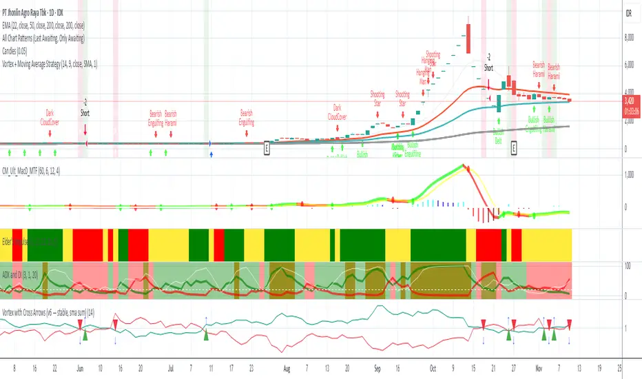
Vortex with Cross Arrows (v6 — stable, sma sum)Vortex Indicators with Cross Arrows, Green cross when VI+ crossing up VI-, and red cross if VI+ crossing below VI-
KillZones & Sessions with AlertsKill Zones & Sessions with Alerts
This TradingView indicator provides comprehensive visualization and alerting for major trading sessions and their associated "kill zones" - periods of high liquidity and price volatility that institutional traders often target.
Based on the great work done by TFlab
Key Features:
1. Four Major Trading Sessions:
Asia Session (2300-0600 UTC) - Sydney + Tokyo markets
London Session (0700-1425 UTC) - Frankfurt + London markets
New York AM Session (1430-1925 UTC)
New York PM Session (1930-2255 UTC)
2. Kill Zones:
Each session includes a "Kill Zone" - the most active trading period within that session:
Asia Kill Zone: 2300-0355 UTC
London Kill Zone: 0700-0955 UTC
NY AM Kill Zone: 1430-1655 UTC
NY PM Kill Zone: 1930-2055 UTC
3. Market Open Zones:
Highlights the first 5 minutes (configurable 1-60 minutes) after each session starts
Shows high/low range with colored boxes and labels
Helps identify initial volatility and price discovery periods
4. Visual Elements:
Session Boxes: Color-coded boxes showing high/low ranges for each session
Kill Zone Overlays: Highlighted areas within sessions showing peak activity times
Dynamic Lines: Track session highs and lows that update as price moves
Optional Volume/Time Info: Display bars, duration, and volume statistics for each session
5. Alert System:
Configurable alerts for session starts (8 total toggles)
Separate alerts for each kill zone start
Once-per-bar frequency to avoid spam
Use Cases:
Identify optimal trading times based on your strategy
Track institutional activity during kill zones
Monitor session breakouts and breakdowns
Set alerts to catch market opens and high-volatility periods
Analyze price behavior across different global markets
The indicator is fully customizable with color coding for each session, toggle switches to show/hide elements, and adjustable market open duration.

5min ORB SICKO ModeThe orb strategy is automated. 5m orb concept is coded into an indicator strategy with multiple settings.

BTC 1h StratUses LuxAlgo-style Support/Resistance levels (pivot-based, with volume break labels).
Adds momentum confirmation (RSI + MACD) to filter fakeouts.Keeps your swing breakout logic (close above swing high / below swing low).
Includes liquidity and TP/SL risk management.

Auto Fibonacci Retracement (Labeled Swings, Rounded Prices)This tool automatically detects the latest confirmed swing high and swing low on your chart, using a user-settable pivot length. It then plots standard Fibonacci retracement levels between these confirmed pivots, labeling each retracement line with its percentage and rounded price for instant reference. All levels update only on swing confirmation, ensuring strict non-repainting logic and transparency.
How it works
Swing Detection:
Uses Pine Script’s native ta.pivothigh and ta.pivotlow functions to locate swing pivots after full confirmation, reducing noise and false signals.
Fibonacci Calculation:
Once two confirmed swings are found, the script draws standard Fibonacci retracement levels (0%, 23.6%, 38.2%, 50%, 61.8%, 78.6%, 100%) between these anchors. The levels adapt to both uptrends and downtrends, based on swing position.
Customization and Clarity:
Users can choose which retracement levels to display and adjust colors, line thickness, styles, and label sizes for chart clarity. All price labels are rounded for improved visibility.
Non-Repainting:
All levels are plotted only after a swing is confirmed by the market; nothing redraws retroactively.
How To Use It
Add the indicator to any chart and timeframe.
Select your preferred pivot length:
Smaller values yield more frequent swings, larger values wait for major structure.
Toggle each Fibonacci level you wish to see in the settings.
Adjust line and label appearance to fit your style.
Interpret retracement levels as potential support/resistance zones, awareness for pullbacks, and context for trend direction.
Combine the indicator with your technical, price action, or volume analysis to plan entries, stops, and targets.
What Traders Should Look For
Visual retracement map between confirmed swings:
Fib lines auto-update as new swings are confirmed, keeping your chart relevant.
Price reaction at Fib levels:
Watch for reversals, consolidations, or continuations near labeled percentages and prices.
Trend assessment:
Quickly spot whether market structure is showing shallow or deep retracements by the distance between levels.
Confluence:
Use retracement levels along with other indicators or market structure for more robust trade setups.
Key Features
Strict non-repainting logic (confirmed swings only)
Configurable retracement levels: Enable/disable each Fib line.
Rounded price & percentage labels
Visual customization: Colors, thickness, line style, label size
Automatic detection of direction (uptrend/downtrend pivots)
Disclaimer
This indicator is a technical analysis and educational tool. It does not provide buy/sell signals, nor guarantee future price movements. Please use in conjunction with your trading plan and risk management.
