light_logLight Log - A Defensive Programming Library for Pine Script
Overview
The Light Log library transforms Pine Script development by introducing structured logging and defensive programming patterns typically found in enterprise languages like C#. This library addresses a fundamental challenge in Pine Script: the lack of sophisticated error handling and debugging tools that developers expect when building complex trading systems.
At its core, Light Log provides three transformative capabilities that work together to create more reliable and maintainable code. First, it wraps all native Pine Script types in error-aware containers, allowing values to carry validation state alongside their data. Second, it offers a comprehensive logging system with severity levels and conditional rendering. Third, it includes defensive programming utilities that catch errors early and make code self-documenting.
The Philosophy of Errors as Values
Traditional Pine Script error handling relies on runtime errors that halt execution, making it difficult to build resilient systems that can gracefully handle edge cases. Light Log introduces a paradigm shift by treating errors as first-class values that flow through your program alongside regular data.
When you wrap a value using Light Log's type system, you're not just storing data – you're creating a container that can carry both the value and its validation state. For example, when you call myNumber.INT() , you receive an INT object that contains both the integer value and a Log object that can describe any issues with that value. This approach, inspired by functional programming languages, allows errors to propagate through calculations without causing immediate failures.
Consider how this changes error handling in practice. Instead of a calculation failing catastrophically when it encounters invalid input, it can produce a result object that contains both the computed value (which might be na) and a detailed log explaining what went wrong. Subsequent operations can check has_error() to decide whether to proceed or handle the error condition gracefully.
The Typed Wrapper System
Light Log provides typed wrappers for every native Pine Script type: INT, FLOAT, BOOL, STRING, COLOR, LINE, LABEL, BOX, TABLE, CHART_POINT, POLYLINE, and LINEFILL. These wrappers serve multiple purposes beyond simple value storage.
Each wrapper type contains two fields: the value field v holds the actual data, while the error field e contains a Log object that tracks the value's validation state. This dual nature enables powerful programming patterns. You can perform operations on wrapped values and accumulate error information along the way, creating an audit trail of how values were processed.
The wrapper system includes convenient methods for converting between wrapped and unwrapped values. The extension methods like INT() , FLOAT() , etc., make it easy to wrap existing values, while the from_INT() , from_FLOAT() methods extract the underlying values when needed. The has_error() method provides a consistent interface for checking whether any wrapped value has encountered issues during processing.
The Log Object: Your Debugging Companion
The Log object represents the heart of Light Log's debugging capabilities. Unlike simple string concatenation for error messages, the Log object provides a structured approach to building, modifying, and rendering diagnostic information.
Each Log object carries three essential pieces of information: an error type (info, warning, error, or runtime_error), a message string that can be built incrementally, and an active flag that controls conditional rendering. This structure enables sophisticated logging patterns where you can build up detailed diagnostic information throughout your script's execution and decide later whether and how to display it.
The Log object's methods support fluent chaining, allowing you to build complex messages in a readable way. The write() and write_line() methods append text to the log, while new_line() adds formatting. The clear() method resets the log for reuse, and the rendering methods ( render_now() , render_condition() , and the general render() ) control when and how messages appear.
Defensive Programming Made Easy
Light Log's argument validation functions transform how you write defensive code. Instead of cluttering your functions with verbose validation logic, you can use concise, self-documenting calls that make your intentions clear.
The argument_error() function provides strict validation that halts execution when conditions aren't met – perfect for catching programming errors early. For less critical issues, argument_log_warning() and argument_log_error() record problems without stopping execution, while argument_log_info() provides debug visibility into your function's behavior.
These functions follow a consistent pattern: they take a condition to check, the function name, the argument name, and a descriptive message. This consistency makes error messages predictable and helpful, automatically formatting them to show exactly where problems occurred.
Building Modular, Reusable Code
Light Log encourages a modular approach to Pine Script development by providing tools that make functions more self-contained and reliable. When functions validate their inputs and return wrapped values with error information, they become true black boxes that can be safely composed into larger systems.
The void_return() function addresses Pine Script's requirement that all code paths return a value, even in error handling branches. This utility function provides a clean way to satisfy the compiler while making it clear that a particular code path should never execute.
The static log pattern, initialized with init_static_log() , enables module-wide error tracking. You can create a persistent Log object that accumulates information across multiple function calls, building a comprehensive diagnostic report that helps you understand complex behaviors in your indicators and strategies.
Real-World Applications
In practice, Light Log shines when building sophisticated trading systems. Imagine developing a complex indicator that processes multiple data streams, performs statistical calculations, and generates trading signals. With Light Log, each processing stage can validate its inputs, perform calculations, and pass along both results and diagnostic information.
For example, a moving average calculation might check that the period is positive, that sufficient data exists, and that the input series contains valid values. Instead of failing silently or throwing runtime errors, it can return a FLOAT object that contains either the calculated average or a detailed explanation of why the calculation couldn't be performed.
Strategy developers benefit even more from Light Log's capabilities. Complex entry and exit logic often involves multiple conditions that must all be satisfied. With Light Log, each condition check can contribute to a comprehensive log that explains exactly why a trade was or wasn't taken, making strategy debugging and optimization much more straightforward.
Performance Considerations
While Light Log adds a layer of abstraction over raw Pine Script values, its design minimizes performance impact. The wrapper objects are lightweight, containing only two fields. The logging operations only consume resources when actually rendered, and the conditional rendering system ensures that production code can run with logging disabled for maximum performance.
The library follows Pine Script best practices for performance, using appropriate data structures and avoiding unnecessary operations. The var keyword in init_static_log() ensures that persistent logs don't create new objects on every bar, maintaining efficiency even in real-time calculations.
Getting Started
Adopting Light Log in your Pine Script projects is straightforward. Import the library, wrap your critical values, add validation to your functions, and use Log objects to track important events. Start small by adding logging to a single function, then expand as you see the benefits of better error visibility and code organization.
Remember that Light Log is designed to grow with your needs. You can use as much or as little of its functionality as makes sense for your project. Even simple uses, like adding argument validation to key functions, can significantly improve code reliability and debugging ease.
Transform your Pine Script development experience with Light Log – because professional trading systems deserve professional development tools.
Light Log Technical Deep Dive: Advanced Patterns and Architecture
Understanding Errors as Values
The concept of "errors as values" represents a fundamental shift in how we think about error handling in Pine Script. In traditional Pine Script development, errors are events – they happen at a specific moment in time and immediately interrupt program flow. Light Log transforms errors into data – they become information that flows through your program just like any other value.
This transformation has profound implications. When errors are values, they can be stored, passed between functions, accumulated, transformed, and inspected. They become part of your program's data flow rather than exceptions to it. This approach, popularized by languages like Rust with its Result type and Haskell with its Either monad, brings functional programming's elegance to Pine Script.
Consider a practical example. Traditional Pine Script might calculate a momentum indicator like this:
momentum = close - close
If period is invalid or if there isn't enough historical data, this calculation might produce na or cause subtle bugs. With Light Log's approach:
calculate_momentum(src, period)=>
result = src.FLOAT()
if period <= 0
result.e.write("Invalid period: must be positive", true, ErrorType.error)
result.v := na
else if bar_index < period
result.e.write("Insufficient data: need " + str.tostring(period) + " bars", true, ErrorType.warning)
result.v := na
else
result.v := src - src
result.e.write("Momentum calculated successfully", false, ErrorType.info)
result
Now the function returns not just a value but a complete computational result that includes diagnostic information. Calling code can make intelligent decisions based on both the value and its associated metadata.
The Monad Pattern in Pine Script
While Pine Script lacks the type system features to implement true monads, Light Log brings monadic thinking to Pine Script development. The wrapped types (INT, FLOAT, etc.) act as computational contexts that carry both values and metadata through a series of transformations.
The key insight of monadic programming is that you can chain operations while automatically propagating context. In Light Log, this context is the error state. When you have a FLOAT that contains an error, operations on that FLOAT can check the error state and decide whether to proceed or propagate the error.
This pattern enables what functional programmers call "railway-oriented programming" – your code follows a success track when all is well but can switch to an error track when problems occur. Both tracks lead to the same destination (a result with error information), but they take different paths based on the validity of intermediate values.
Composable Error Handling
Light Log's design encourages composition – building complex functionality from simpler, well-tested components. Each component can validate its inputs, perform its calculation, and return a result with appropriate error information. Higher-level functions can then combine these results intelligently.
Consider building a complex trading signal from multiple indicators:
generate_signal(src, fast_period, slow_period, signal_period) =>
log = init_static_log(ErrorType.info)
// Calculate components with error tracking
fast_ma = calculate_ma(src, fast_period)
slow_ma = calculate_ma(src, slow_period)
// Check for errors in components
if fast_ma.has_error()
log.write_line("Fast MA error: " + fast_ma.e.message, true)
if slow_ma.has_error()
log.write_line("Slow MA error: " + slow_ma.e.message, true)
// Proceed with calculation if no errors
signal = 0.0.FLOAT()
if not (fast_ma.has_error() or slow_ma.has_error())
macd_line = fast_ma.v - slow_ma.v
signal_line = calculate_ma(macd_line, signal_period)
if signal_line.has_error()
log.write_line("Signal line error: " + signal_line.e.message, true)
signal.e := log
else
signal.v := macd_line - signal_line.v
log.write("Signal generated successfully")
else
signal.e := log
signal.v := na
signal
This composable approach makes complex calculations more reliable and easier to debug. Each component is responsible for its own validation and error reporting, and the composite function orchestrates these components while maintaining comprehensive error tracking.
The Static Log Pattern
The init_static_log() function introduces a powerful pattern for maintaining state across function calls. In Pine Script, the var keyword creates variables that persist across bars but are initialized only once. Light Log leverages this to create logging objects that can accumulate information throughout a script's execution.
This pattern is particularly valuable for debugging complex strategies where you need to understand behavior across multiple bars. You can create module-level logs that track important events:
// Module-level diagnostic log
diagnostics = init_static_log(ErrorType.info)
// Track strategy decisions across bars
check_entry_conditions() =>
diagnostics.clear() // Start fresh each bar
diagnostics.write_line("Bar " + str.tostring(bar_index) + " analysis:")
if close > sma(close, 20)
diagnostics.write_line("Price above SMA20", false)
else
diagnostics.write_line("Price below SMA20 - no entry", true, ErrorType.warning)
if volume > sma(volume, 20) * 1.5
diagnostics.write_line("Volume surge detected", false)
else
diagnostics.write_line("Normal volume", false)
// Render diagnostics based on verbosity setting
if debug_mode
diagnostics.render_now()
Advanced Validation Patterns
Light Log's argument validation functions enable sophisticated precondition checking that goes beyond simple null checks. You can implement complex validation logic while keeping your code readable:
validate_price_data(open_val, high_val, low_val, close_val) =>
argument_error(na(open_val) or na(high_val) or na(low_val) or na(close_val),
"validate_price_data", "OHLC values", "contain na values")
argument_error(high_val < low_val,
"validate_price_data", "high/low", "high is less than low")
argument_error(close_val > high_val or close_val < low_val,
"validate_price_data", "close", "is outside high/low range")
argument_log_warning(high_val == low_val,
"validate_price_data", "high/low", "are equal (no range)")
This validation function documents its requirements clearly and fails fast with helpful error messages when assumptions are violated. The mix of errors (which halt execution) and warnings (which allow continuation) provides fine-grained control over how strict your validation should be.
Performance Optimization Strategies
While Light Log adds abstraction, careful design minimizes overhead. Understanding Pine Script's execution model helps you use Light Log efficiently.
Pine Script executes once per bar, so operations that seem expensive in traditional programming might have negligible impact. However, when building real-time systems, every optimization matters. Light Log provides several patterns for efficient use:
Lazy Evaluation: Log messages are only built when they'll be rendered. Use conditional logging to avoid string concatenation in production:
if debug_mode
log.write_line("Calculated value: " + str.tostring(complex_calculation))
Selective Wrapping: Not every value needs error tracking. Wrap values at API boundaries and critical calculation points, but use raw values for simple operations:
// Wrap at boundaries
input_price = close.FLOAT()
validated_period = validate_period(input_period).INT()
// Use raw values internally
sum = 0.0
for i = 0 to validated_period.v - 1
sum += close
Error Propagation: When errors occur early, avoid expensive calculations:
process_data(input) =>
validated = validate_input(input)
if validated.has_error()
validated // Return early with error
else
// Expensive processing only if valid
perform_complex_calculation(validated)
Integration Patterns
Light Log integrates smoothly with existing Pine Script code. You can adopt it incrementally, starting with critical functions and expanding coverage as needed.
Boundary Validation: Add Light Log at the boundaries of your system – where user input enters and where final outputs are produced. This catches most errors while minimizing changes to existing code.
Progressive Enhancement: Start by adding argument validation to existing functions. Then wrap return values. Finally, add comprehensive logging. Each step improves reliability without requiring a complete rewrite.
Testing and Debugging: Use Light Log's conditional rendering to create debug modes for your scripts. Production users see clean output while developers get detailed diagnostics:
// User input for debug mode
debug = input.bool(false, "Enable debug logging")
// Conditional diagnostic output
if debug
diagnostics.render_now()
else
diagnostics.render_condition() // Only shows errors/warnings
Future-Proofing Your Code
Light Log's patterns prepare your code for Pine Script's evolution. As Pine Script adds more sophisticated features, code that uses structured error handling and defensive programming will adapt more easily than code that relies on implicit assumptions.
The type wrapper system, in particular, positions your code to take advantage of potential future features or more sophisticated type inference. By thinking in terms of wrapped values and error propagation today, you're building code that will remain maintainable and extensible tomorrow.
Light Log doesn't just make your Pine Script better today – it prepares it for the trading systems you'll need to build tomorrow.
Library "light_log"
A lightweight logging and defensive programming library for Pine Script.
Designed for modular and extensible scripts, this utility provides structured runtime validation,
conditional logging, and reusable `Log` objects for centralized error propagation.
It also introduces a typed wrapping system for all native Pine values (e.g., `INT`, `FLOAT`, `LABEL`),
allowing values to carry errors alongside data. This enables functional-style flows with built-in
validation tracking, error detection (`has_error()`), and fluent chaining.
Inspired by structured logging patterns found in systems like C#, it reduces boilerplate,
enforces argument safety, and encourages clean, maintainable code architecture.
method INT(self, error_type)
Wraps an `int` value into an `INT` struct with an optional log severity.
Namespace types: series int, simple int, input int, const int
Parameters:
self (int) : The raw `int` value to wrap.
error_type (series ErrorType) : Optional severity level to associate with the log. Default is `ErrorType.error`.
Returns: An `INT` object containing the value and a default Log instance.
method FLOAT(self, error_type)
Wraps a `float` value into a `FLOAT` struct with an optional log severity.
Namespace types: series float, simple float, input float, const float
Parameters:
self (float) : The raw `float` value to wrap.
error_type (series ErrorType) : Optional severity level to associate with the log. Default is `ErrorType.error`.
Returns: A `FLOAT` object containing the value and a default Log instance.
method BOOL(self, error_type)
Wraps a `bool` value into a `BOOL` struct with an optional log severity.
Namespace types: series bool, simple bool, input bool, const bool
Parameters:
self (bool) : The raw `bool` value to wrap.
error_type (series ErrorType) : Optional severity level to associate with the log. Default is `ErrorType.error`.
Returns: A `BOOL` object containing the value and a default Log instance.
method STRING(self, error_type)
Wraps a `string` value into a `STRING` struct with an optional log severity.
Namespace types: series string, simple string, input string, const string
Parameters:
self (string) : The raw `string` value to wrap.
error_type (series ErrorType) : Optional severity level to associate with the log. Default is `ErrorType.error`.
Returns: A `STRING` object containing the value and a default Log instance.
method COLOR(self, error_type)
Wraps a `color` value into a `COLOR` struct with an optional log severity.
Namespace types: series color, simple color, input color, const color
Parameters:
self (color) : The raw `color` value to wrap.
error_type (series ErrorType) : Optional severity level to associate with the log. Default is `ErrorType.error`.
Returns: A `COLOR` object containing the value and a default Log instance.
method LINE(self, error_type)
Wraps a `line` object into a `LINE` struct with an optional log severity.
Namespace types: series line
Parameters:
self (line) : The raw `line` object to wrap.
error_type (series ErrorType) : Optional severity level to associate with the log. Default is `ErrorType.error`.
Returns: A `LINE` object containing the value and a default Log instance.
method LABEL(self, error_type)
Wraps a `label` object into a `LABEL` struct with an optional log severity.
Namespace types: series label
Parameters:
self (label) : The raw `label` object to wrap.
error_type (series ErrorType) : Optional severity level to associate with the log. Default is `ErrorType.error`.
Returns: A `LABEL` object containing the value and a default Log instance.
method BOX(self, error_type)
Wraps a `box` object into a `BOX` struct with an optional log severity.
Namespace types: series box
Parameters:
self (box) : The raw `box` object to wrap.
error_type (series ErrorType) : Optional severity level to associate with the log. Default is `ErrorType.error`.
Returns: A `BOX` object containing the value and a default Log instance.
method TABLE(self, error_type)
Wraps a `table` object into a `TABLE` struct with an optional log severity.
Namespace types: series table
Parameters:
self (table) : The raw `table` object to wrap.
error_type (series ErrorType) : Optional severity level to associate with the log. Default is `ErrorType.error`.
Returns: A `TABLE` object containing the value and a default Log instance.
method CHART_POINT(self, error_type)
Wraps a `chart.point` value into a `CHART_POINT` struct with an optional log severity.
Namespace types: chart.point
Parameters:
self (chart.point) : The raw `chart.point` value to wrap.
error_type (series ErrorType) : Optional severity level to associate with the log. Default is `ErrorType.error`.
Returns: A `CHART_POINT` object containing the value and a default Log instance.
method POLYLINE(self, error_type)
Wraps a `polyline` object into a `POLYLINE` struct with an optional log severity.
Namespace types: series polyline, series polyline, series polyline, series polyline
Parameters:
self (polyline) : The raw `polyline` object to wrap.
error_type (series ErrorType) : Optional severity level to associate with the log. Default is `ErrorType.error`.
Returns: A `POLYLINE` object containing the value and a default Log instance.
method LINEFILL(self, error_type)
Wraps a `linefill` object into a `LINEFILL` struct with an optional log severity.
Namespace types: series linefill
Parameters:
self (linefill) : The raw `linefill` object to wrap.
error_type (series ErrorType) : Optional severity level to associate with the log. Default is `ErrorType.error`.
Returns: A `LINEFILL` object containing the value and a default Log instance.
method from_INT(self)
Extracts the integer value from an INT wrapper.
Namespace types: INT
Parameters:
self (INT) : The wrapped INT instance.
Returns: The underlying `int` value.
method from_FLOAT(self)
Extracts the float value from a FLOAT wrapper.
Namespace types: FLOAT
Parameters:
self (FLOAT) : The wrapped FLOAT instance.
Returns: The underlying `float` value.
method from_BOOL(self)
Extracts the boolean value from a BOOL wrapper.
Namespace types: BOOL
Parameters:
self (BOOL) : The wrapped BOOL instance.
Returns: The underlying `bool` value.
method from_STRING(self)
Extracts the string value from a STRING wrapper.
Namespace types: STRING
Parameters:
self (STRING) : The wrapped STRING instance.
Returns: The underlying `string` value.
method from_COLOR(self)
Extracts the color value from a COLOR wrapper.
Namespace types: COLOR
Parameters:
self (COLOR) : The wrapped COLOR instance.
Returns: The underlying `color` value.
method from_LINE(self)
Extracts the line object from a LINE wrapper.
Namespace types: LINE
Parameters:
self (LINE) : The wrapped LINE instance.
Returns: The underlying `line` object.
method from_LABEL(self)
Extracts the label object from a LABEL wrapper.
Namespace types: LABEL
Parameters:
self (LABEL) : The wrapped LABEL instance.
Returns: The underlying `label` object.
method from_BOX(self)
Extracts the box object from a BOX wrapper.
Namespace types: BOX
Parameters:
self (BOX) : The wrapped BOX instance.
Returns: The underlying `box` object.
method from_TABLE(self)
Extracts the table object from a TABLE wrapper.
Namespace types: TABLE
Parameters:
self (TABLE) : The wrapped TABLE instance.
Returns: The underlying `table` object.
method from_CHART_POINT(self)
Extracts the chart.point from a CHART_POINT wrapper.
Namespace types: CHART_POINT
Parameters:
self (CHART_POINT) : The wrapped CHART_POINT instance.
Returns: The underlying `chart.point` value.
method from_POLYLINE(self)
Extracts the polyline object from a POLYLINE wrapper.
Namespace types: POLYLINE
Parameters:
self (POLYLINE) : The wrapped POLYLINE instance.
Returns: The underlying `polyline` object.
method from_LINEFILL(self)
Extracts the linefill object from a LINEFILL wrapper.
Namespace types: LINEFILL
Parameters:
self (LINEFILL) : The wrapped LINEFILL instance.
Returns: The underlying `linefill` object.
method has_error(self)
Returns true if the INT wrapper has an active log entry.
Namespace types: INT
Parameters:
self (INT) : The INT instance to check.
Returns: True if an error or message is active in the log.
method has_error(self)
Returns true if the FLOAT wrapper has an active log entry.
Namespace types: FLOAT
Parameters:
self (FLOAT) : The FLOAT instance to check.
Returns: True if an error or message is active in the log.
method has_error(self)
Returns true if the BOOL wrapper has an active log entry.
Namespace types: BOOL
Parameters:
self (BOOL) : The BOOL instance to check.
Returns: True if an error or message is active in the log.
method has_error(self)
Returns true if the STRING wrapper has an active log entry.
Namespace types: STRING
Parameters:
self (STRING) : The STRING instance to check.
Returns: True if an error or message is active in the log.
method has_error(self)
Returns true if the COLOR wrapper has an active log entry.
Namespace types: COLOR
Parameters:
self (COLOR) : The COLOR instance to check.
Returns: True if an error or message is active in the log.
method has_error(self)
Returns true if the LINE wrapper has an active log entry.
Namespace types: LINE
Parameters:
self (LINE) : The LINE instance to check.
Returns: True if an error or message is active in the log.
method has_error(self)
Returns true if the LABEL wrapper has an active log entry.
Namespace types: LABEL
Parameters:
self (LABEL) : The LABEL instance to check.
Returns: True if an error or message is active in the log.
method has_error(self)
Returns true if the BOX wrapper has an active log entry.
Namespace types: BOX
Parameters:
self (BOX) : The BOX instance to check.
Returns: True if an error or message is active in the log.
method has_error(self)
Returns true if the TABLE wrapper has an active log entry.
Namespace types: TABLE
Parameters:
self (TABLE) : The TABLE instance to check.
Returns: True if an error or message is active in the log.
method has_error(self)
Returns true if the CHART_POINT wrapper has an active log entry.
Namespace types: CHART_POINT
Parameters:
self (CHART_POINT) : The CHART_POINT instance to check.
Returns: True if an error or message is active in the log.
method has_error(self)
Returns true if the POLYLINE wrapper has an active log entry.
Namespace types: POLYLINE
Parameters:
self (POLYLINE) : The POLYLINE instance to check.
Returns: True if an error or message is active in the log.
method has_error(self)
Returns true if the LINEFILL wrapper has an active log entry.
Namespace types: LINEFILL
Parameters:
self (LINEFILL) : The LINEFILL instance to check.
Returns: True if an error or message is active in the log.
void_return()
Utility function used when a return is syntactically required but functionally unnecessary.
Returns: Nothing. Function never executes its body.
argument_error(condition, function, argument, message)
Throws a runtime error when a condition is met. Used for strict argument validation.
Parameters:
condition (bool) : Boolean expression that triggers the runtime error.
function (string) : Name of the calling function (for formatting).
argument (string) : Name of the problematic argument.
message (string) : Description of the error cause.
Returns: Never returns. Halts execution if the condition is true.
argument_log_info(condition, function, argument, message)
Logs an informational message when a condition is met. Used for optional debug visibility.
Parameters:
condition (bool) : Boolean expression that triggers the log.
function (string) : Name of the calling function.
argument (string) : Argument name being referenced.
message (string) : Informational message to log.
Returns: Nothing. Logs if the condition is true.
argument_log_warning(condition, function, argument, message)
Logs a warning when a condition is met. Non-fatal but highlights potential issues.
Parameters:
condition (bool) : Boolean expression that triggers the warning.
function (string) : Name of the calling function.
argument (string) : Argument name being referenced.
message (string) : Warning message to log.
Returns: Nothing. Logs if the condition is true.
argument_log_error(condition, function, argument, message)
Logs an error message when a condition is met. Does not halt execution.
Parameters:
condition (bool) : Boolean expression that triggers the error log.
function (string) : Name of the calling function.
argument (string) : Argument name being referenced.
message (string) : Error message to log.
Returns: Nothing. Logs if the condition is true.
init_static_log(error_type, message, active)
Initializes a persistent (var) Log object. Ideal for global logging in scripts or modules.
Parameters:
error_type (series ErrorType) : Initial severity level (required).
message (string) : Optional starting message string. Default value of ("").
active (bool) : Whether the log should be flagged active on initialization. Default value of (false).
Returns: A static Log object with the given parameters.
method new_line(self)
Appends a newline character to the Log message. Useful for separating entries during chained writes.
Namespace types: Log
Parameters:
self (Log) : The Log instance to modify.
Returns: The updated Log object with a newline appended.
method write(self, message, flag_active, error_type)
Appends a message to a Log object without a newline. Updates severity and active state if specified.
Namespace types: Log
Parameters:
self (Log) : The Log instance being modified.
message (string) : The text to append to the log.
flag_active (bool) : Whether to activate the log for conditional rendering. Default value of (false).
error_type (series ErrorType) : Optional override for the severity level. Default value of (na).
Returns: The updated Log object.
method write_line(self, message, flag_active, error_type)
Appends a message to a Log object, prefixed with a newline for clarity.
Namespace types: Log
Parameters:
self (Log) : The Log instance being modified.
message (string) : The text to append to the log.
flag_active (bool) : Whether to activate the log for conditional rendering. Default value of (false).
error_type (series ErrorType) : Optional override for the severity level. Default value of (na).
Returns: The updated Log object.
method clear(self, flag_active, error_type)
Clears a Log object’s message and optionally reactivates it. Can also update the error type.
Namespace types: Log
Parameters:
self (Log) : The Log instance being cleared.
flag_active (bool) : Whether to activate the log after clearing. Default value of (false).
error_type (series ErrorType) : Optional new error type to assign. If not provided, the previous type is retained. Default value of (na).
Returns: The cleared Log object.
method render_condition(self, flag_active, error_type)
Conditionally renders the log if it is active. Allows overriding error type and controlling active state afterward.
Namespace types: Log
Parameters:
self (Log) : The Log instance to evaluate and render.
flag_active (bool) : Whether to activate the log after rendering. Default value of (false).
error_type (series ErrorType) : Optional error type override. Useful for contextual formatting just before rendering. Default value of (na).
Returns: The updated Log object.
method render_now(self, flag_active, error_type)
Immediately renders the log regardless of `active` state. Allows overriding error type and active flag.
Namespace types: Log
Parameters:
self (Log) : The Log instance to render.
flag_active (bool) : Whether to activate the log after rendering. Default value of (false).
error_type (series ErrorType) : Optional error type override. Allows dynamic severity adjustment at render time. Default value of (na).
Returns: The updated Log object.
render(self, condition, flag_active, error_type)
Renders the log conditionally or unconditionally. Allows full control over render behavior.
Parameters:
self (Log) : The Log instance to render.
condition (bool) : If true, renders only if the log is active. If false, always renders. Default value of (false).
flag_active (bool) : Whether to activate the log after rendering. Default value of (false).
error_type (series ErrorType) : Optional error type override passed to the render methods. Default value of (na).
Returns: The updated Log object.
Log
A structured object used to store and render logging messages.
Fields:
error_type (series ErrorType) : The severity level of the message (from the ErrorType enum).
message (series string) : The text of the log message.
active (series bool) : Whether the log should trigger rendering when conditionally evaluated.
INT
A wrapped integer type with attached logging for validation or tracing.
Fields:
v (series int) : The underlying `int` value.
e (Log) : Optional log object describing validation status or error context.
FLOAT
A wrapped float type with attached logging for validation or tracing.
Fields:
v (series float) : The underlying `float` value.
e (Log) : Optional log object describing validation status or error context.
BOOL
A wrapped boolean type with attached logging for validation or tracing.
Fields:
v (series bool) : The underlying `bool` value.
e (Log) : Optional log object describing validation status or error context.
STRING
A wrapped string type with attached logging for validation or tracing.
Fields:
v (series string) : The underlying `string` value.
e (Log) : Optional log object describing validation status or error context.
COLOR
A wrapped color type with attached logging for validation or tracing.
Fields:
v (series color) : The underlying `color` value.
e (Log) : Optional log object describing validation status or error context.
LINE
A wrapped line object with attached logging for validation or tracing.
Fields:
v (series line) : The underlying `line` value.
e (Log) : Optional log object describing validation status or error context.
LABEL
A wrapped label object with attached logging for validation or tracing.
Fields:
v (series label) : The underlying `label` value.
e (Log) : Optional log object describing validation status or error context.
BOX
A wrapped box object with attached logging for validation or tracing.
Fields:
v (series box) : The underlying `box` value.
e (Log) : Optional log object describing validation status or error context.
TABLE
A wrapped table object with attached logging for validation or tracing.
Fields:
v (series table) : The underlying `table` value.
e (Log) : Optional log object describing validation status or error context.
CHART_POINT
A wrapped chart point with attached logging for validation or tracing.
Fields:
v (chart.point) : The underlying `chart.point` value.
e (Log) : Optional log object describing validation status or error context.
POLYLINE
A wrapped polyline object with attached logging for validation or tracing.
Fields:
v (series polyline) : The underlying `polyline` value.
e (Log) : Optional log object describing validation status or error context.
LINEFILL
A wrapped linefill object with attached logging for validation or tracing.
Fields:
v (series linefill) : The underlying `linefill` value.
e (Log) : Optional log object describing validation status or error context.
Indicators and strategies
Multifractal Forecast [ScorsoneEnterprises]Multifractal Forecast Indicator
The Multifractal Forecast is an indicator designed to model and forecast asset price movements using a multifractal framework. It uses concepts from fractal geometry and stochastic processes, specifically the Multifractal Model of Asset Returns (MMAR) and fractional Brownian motion (fBm), to generate price forecasts based on historical price data. The indicator visualizes potential future price paths as colored lines, providing traders with a probabilistic view of price trends over a specified trading time scale. Below is a detailed breakdown of the indicator’s functionality, inputs, calculations, and visualization.
Overview
Purpose: The indicator forecasts future price movements by simulating multiple price paths based on a multifractal model, which accounts for the complex, non-linear behavior of financial markets.
Key Concepts:
Multifractal Model of Asset Returns (MMAR): Models price movements as a multifractal process, capturing varying degrees of volatility and self-similarity across different time scales.
Fractional Brownian Motion (fBm): A generalization of Brownian motion that incorporates long-range dependence and self-similarity, controlled by the Hurst exponent.
Binomial Cascade: Used to model trading time, introducing heterogeneity in time scales to reflect market activity bursts.
Hurst Exponent: Measures the degree of long-term memory in the price series (persistence, randomness, or mean-reversion).
Rescaled Range (R/S) Analysis: Estimates the Hurst exponent to quantify the fractal nature of the price series.
Inputs
The indicator allows users to customize its behavior through several input parameters, each influencing the multifractal model and forecast generation:
Maximum Lag (max_lag):
Type: Integer
Default: 50
Minimum: 5
Purpose: Determines the maximum lag used in the rescaled range (R/S) analysis to calculate the Hurst exponent. A higher lag increases the sample size for Hurst estimation but may smooth out short-term dynamics.
2 to the n values in the Multifractal Model (n):
Type: Integer
Default: 4
Purpose: Defines the resolution of the multifractal model by setting the size of arrays used in calculations (N = 2^n). For example, n=4 results in N=16 data points. Larger n increases computational complexity and detail but may exceed Pine Script’s array size limits (capped at 100,000).
Multiplier for Binomial Cascade (m):
Type: Float
Default: 0.8
Purpose: Controls the asymmetry in the binomial cascade, which models trading time. The multiplier m (and its complement 2.0 - m) determines how mass is distributed across time scales. Values closer to 1 create more balanced cascades, while values further from 1 introduce more variability.
Length Scale for fBm (L):
Type: Float
Default: 100,000.0
Purpose: Scales the fractional Brownian motion output, affecting the amplitude of simulated price paths. Larger values increase the magnitude of forecasted price movements.
Cumulative Sum (cum):
Type: Integer (0 or 1)
Default: 1
Purpose: Toggles whether the fBm output is cumulatively summed (1=On, 0=Off). When enabled, the fBm series is accumulated to simulate a price path with memory, resembling a random walk with long-range dependence.
Trading Time Scale (T):
Type: Integer
Default: 5
Purpose: Defines the forecast horizon in bars (20 bars into the future). It also scales the binomial cascade’s output to align with the desired trading time frame.
Number of Simulations (num_simulations):
Type: Integer
Default: 5
Minimum: 1
Purpose: Specifies how many forecast paths are simulated and plotted. More simulations provide a broader range of possible price outcomes but increase computational load.
Core Calculations
The indicator combines several mathematical and statistical techniques to generate price forecasts. Below is a step-by-step explanation of its calculations:
Log Returns (lgr):
The indicator calculates log returns as math.log(close / close ) when both the current and previous close prices are positive. This measures the relative price change in a logarithmic scale, which is standard for financial time series analysis to stabilize variance.
Hurst Exponent Estimation (get_hurst_exponent):
Purpose: Estimates the Hurst exponent (H) to quantify the degree of long-term memory in the price series.
Method: Uses rescaled range (R/S) analysis:
For each lag from 2 to max_lag, the function calc_rescaled_range computes the rescaled range:
Calculate the mean of the log returns over the lag period.
Compute the cumulative deviation from the mean.
Find the range (max - min) of the cumulative deviation.
Divide the range by the standard deviation of the log returns to get the rescaled range.
The log of the rescaled range (log(R/S)) is regressed against the log of the lag (log(lag)) using the polyfit_slope function.
The slope of this regression is the Hurst exponent (H).
Interpretation:
H = 0.5: Random walk (no memory, like standard Brownian motion).
H > 0.5: Persistent behavior (trends tend to continue).
H < 0.5: Mean-reverting behavior (price tends to revert to the mean).
Fractional Brownian Motion (get_fbm):
Purpose: Generates a fractional Brownian motion series to model price movements with long-range dependence.
Inputs: n (array size 2^n), H (Hurst exponent), L (length scale), cum (cumulative sum toggle).
Method:
Computes covariance for fBm using the formula: 0.5 * (|i+1|^(2H) - 2 * |i|^(2H) + |i-1|^(2H)).
Uses Hosking’s method (referenced from Columbia University’s implementation) to generate fBm:
Initializes arrays for covariance (cov), intermediate calculations (phi, psi), and output.
Iteratively computes the fBm series by incorporating a random term scaled by the variance (v) and covariance structure.
Applies scaling based on L / N^H to adjust the amplitude.
Optionally applies cumulative summation if cum = 1 to produce a path with memory.
Output: An array of 2^n values representing the fBm series.
Binomial Cascade (get_binomial_cascade):
Purpose: Models trading time (theta) to account for non-uniform market activity (e.g., bursts of volatility).
Inputs: n (array size 2^n), m (multiplier), T (trading time scale).
Method:
Initializes an array of size 2^n with values of 1.0.
Iteratively applies a binomial cascade:
For each block (from 0 to n-1), splits the array into segments.
Randomly assigns a multiplier (m or 2.0 - m) to each segment, redistributing mass.
Normalizes the array by dividing by its sum and scales by T.
Checks for array size limits to prevent Pine Script errors.
Output: An array (theta) representing the trading time, which warps the fBm to reflect market activity.
Interpolation (interpolate_fbm):
Purpose: Maps the fBm series to the trading time scale to produce a forecast.
Method:
Computes the cumulative sum of theta and normalizes it to .
Interpolates the fBm series linearly based on the normalized trading time.
Ensures the output aligns with the trading time scale (T).
Output: An array of interpolated fBm values representing log returns over the forecast horizon.
Price Path Generation:
For each simulation (up to num_simulations):
Generates an fBm series using get_fbm.
Interpolates it with the trading time (theta) using interpolate_fbm.
Converts log returns to price levels:
Starts with the current close price.
For each step i in the forecast horizon (T), computes the price as prev_price * exp(log_return).
Output: An array of price levels for each simulation.
Visualization:
Trigger: Updates every T bars when the bar state is confirmed (barstate.isconfirmed).
Process:
Clears previous lines from line_array.
For each simulation, plots a line from the current bar’s close price to the forecasted price at bar_index + T.
Colors the line using a gradient (color.from_gradient) based on the final forecasted price relative to the minimum and maximum forecasted prices across all simulations (red for lower prices, teal for higher prices).
Output: Multiple colored lines on the chart, each representing a possible price path over the next T bars.
How It Works on the Chart
Initialization: On each bar, the indicator calculates the Hurst exponent (H) using historical log returns and prepares the trading time (theta) using the binomial cascade.
Forecast Generation: Every T bars, it generates num_simulations price paths:
Each path starts at the current close price.
Uses fBm to model log returns, warped by the trading time.
Converts log returns to price levels.
Plotting: Draws lines from the current bar to the forecasted price T bars ahead, with colors indicating relative price levels.
Dynamic Updates: The forecast updates every T bars, replacing old lines with new ones based on the latest price data and calculations.
Key Features
Multifractal Modeling: Captures complex market dynamics by combining fBm (long-range dependence) with a binomial cascade (non-uniform time).
Customizable Parameters: Allows users to adjust the forecast horizon, model resolution, scaling, and number of simulations.
Probabilistic Forecast: Multiple simulations provide a range of possible price outcomes, helping traders assess uncertainty.
Visual Clarity: Gradient-colored lines make it easy to distinguish bullish (teal) and bearish (red) forecasts.
Potential Use Cases
Trend Analysis: Identify potential price trends or reversals based on the direction and spread of forecast lines.
Risk Assessment: Evaluate the range of possible price outcomes to gauge market uncertainty.
Volatility Analysis: The Hurst exponent and binomial cascade provide insights into market persistence and volatility clustering.
Limitations
Computational Intensity: Large values of n or num_simulations may slow down execution or hit Pine Script’s array size limits.
Randomness: The binomial cascade and fBm rely on random terms (math.random), which may lead to variability between runs.
Assumptions: The model assumes log-normal price movements and fractal behavior, which may not always hold in extreme market conditions.
Adjusting Inputs:
Set max_lag based on the desired depth of historical analysis.
Adjust n for model resolution (start with 4–6 to avoid performance issues).
Tune m to control trading time variability (0.5–1.5 is typical).
Set L to scale the forecast amplitude (experiment with values like 10,000–1,000,000).
Choose T based on your trading horizon (20 for short-term, 50 for longer-term for example).
Select num_simulations for the number of forecast paths (5–10 is reasonable for visualization).
Interpret Output:
Teal lines suggest bullish scenarios, red lines suggest bearish scenarios.
A wide spread of lines indicates high uncertainty; convergence suggests a stronger trend.
Monitor Updates: Forecasts update every T bars, so check the chart periodically for new projections.
Chart Examples
This is a daily AMEX:SPY chart with default settings. We see the simulations being done every T bars and they provide a range for us to analyze with a few simulations still in the range.
On this intraday PEPPERSTONE:COCOA chart I modified the Length Scale for fBm, L, parameter to be 1000 from 100000. Adjusting the parameter as you switch between timeframes can give you more contextual simulations.
On BITSTAMP:ETHUSD I modified the L to be 1000000 to have a more contextual set of simulations with crypto's volatile nature.
With L at 100000 we see the range for NASDAQ:TLT is correctly simulated. The recent pop stays within the bounds of the highest simulation. Note this is a cherry picked example to show the power and potential of these simulations.
Technical Notes
Error Handling: The script includes checks for array size limits and division by zero (math.abs(denominator) > 1e-10, v := math.max(v, 1e-10)).
External Reference: The fBm implementation is based on Hosking’s method (www.columbia.edu), ensuring a robust algorithm.
Conclusion
The Multifractal Forecast is a powerful tool for traders seeking to model complex market dynamics using a multifractal framework. By combining fBm, binomial cascades, and Hurst exponent analysis, it generates probabilistic price forecasts that account for long-range dependence and non-uniform market activity. Its customizable inputs and clear visualizations make it suitable for both technical analysis and strategy development, though users should be mindful of its computational demands and parameter sensitivity. For optimal use, experiment with input settings and validate forecasts against other technical indicators or market conditions.
Futures Margin Lookup TableThis script applies a table to your chart, which provides the intraday and overnight margin requirements of the currently selected symbol.
In this indicator the user must provide the broker data in the form of specifically formatted text blocks. The data for which should be found on the broker website under futures margin requirements.
The purpose for it's creation is due to the non-standard way each individual broker may price their margins and lack of information within TradingView when connected to some (maybe all) brokers, including during paper trading, as the flat percentage rule is not accurate.
An example of information could look like this
MES;Micro S&P;$50;$2406
ES;E-Mini S&P;$500;$24,053
GC;Gold;$500;$16500
NQ;E-Mini Nasdaq;$1,000;$34,810
FDAX;Dax Index;€2,000;€44,311
Each symbol begins a new line, and the values on that line are separated by semicolons (;)
Each line consists of the following...
SYMBOL : Search string used to match to the beginning of the current chart symbol.
NAME: Human readable name
INTRA: Intraday trading margin requirement per contract
OVERNIGHT: Overnight trading margin requirement per contract
The script simply finds a matching line within your provided information using the current chart symbol.
So for example the continuous chart for
NQ1!
would match to the user specified line starting with NQ... as would the individual contract dates such as NQM2025, NQK2025, etc.
NOTES:
There is a possibility that symbols with similar starting characters could match. If this is the case put the longer symbol higher in the list.
There is also a line / character limit to the text input fields within pinescript. Ensure the text you enter / paste into them is not truncated. If so there are 3 input fields for just this purpose. Find the last complete line and continue the remaining symbol lines on the subsequent inputs.
Hme Rolling VolumeThis indicator allows you to display volume in a continious rolling time frame.
Instead of starting at zero for each new bar, it displays, for example, the cumulative volume of the last 120 seconds on a 2-minute chart.
This helps you track volume trends even more quickly and interpret their behavior without the break between bars.

Fibonacci Entry Bands [AlgoAlpha]OVERVIEW
This script plots Fibonacci Entry Bands, a trend-following and mean-reversion hybrid system built around dynamic volatility-adjusted bands scaled using key Fibonacci levels. It calculates a smoothed basis line and overlays multiple bands at fixed Fibonacci multipliers of either ATR or standard deviation. Depending on the trend direction, specific upper or lower bands become active, offering a clear framework for entry timing, trend identification, and profit-taking zones.
CONCEPTS
The core idea is to use Fibonacci levels—0.618, 1.0, 1.618, and 2.618—as multipliers on a volatility measure to form layered price bands around a trend-following moving average. Trends are defined by whether the basis is rising or falling. The trend determines which side of the bands is emphasized: upper bands for downtrends, lower bands for uptrends. This approach captures both directional bias and extreme price extensions. Take-profit logic is built in via crossovers relative to the outermost bands, scaled by user-selected aggressiveness.
FEATURES
Basis Line – A double EMA smoothing of the source defines trend direction and acts as the central mean.
Volatility Bands – Four levels per side (based on selected ATR or stdev) mark the Fibonacci bands. These become visible only when trend direction matches the side (e.g., only lower bands plot in an uptrend).
Bar Coloring – Bars are shaded with adjustable transparency depending on distance from the basis, with color intensity helping gauge overextension.
Entry Arrows – A trend shift triggers either a long or short signal, with a marker at the outermost band with ▲/▼ signs.
Take-Profit Crosses – If price rejects near the outer band (based on aggressiveness setting), a cross appears marking potential profit-taking.
Bounce Signals – Minor pullbacks that respect the basis line are marked with triangle arrows, hinting at continuation setups.
Customization – Users can toggle bar coloring, signal markers, and select between ATR/stdev as well as take-profit aggressiveness.
Alerts – All major signals, including entries, take-profits, and bounces, are available as alert conditions.
USAGE
To use this tool, load it on your chart, adjust the inputs for volatility method and aggressiveness, and wait for entries to form on trend changes. Use TP crosses and bounce arrows as potential exit or scale-in signals.

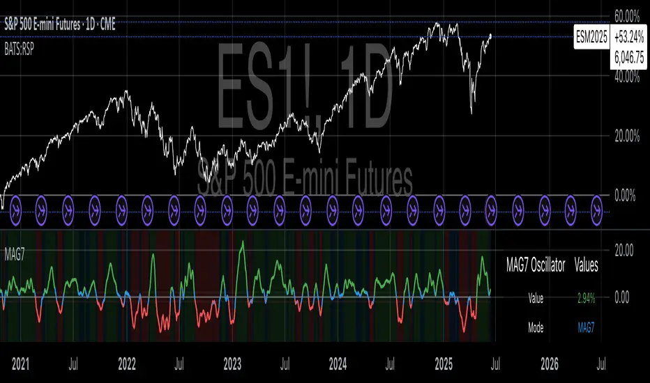
Magnificent 7 OscillatorThe Magnificent 7 Oscillator is a sophisticated momentum-based technical indicator designed to analyze the collective performance of the seven largest technology companies in the U.S. stock market (Apple, Microsoft, Alphabet, Amazon, NVIDIA, Tesla, and Meta). This indicator incorporates established momentum factor research and provides three distinct analytical modes: absolute momentum tracking, equal-weighted market comparison, and relative performance analysis. The tool integrates five different oscillator methodologies and includes advanced breadth analysis capabilities.
Theoretical Foundation
Momentum Factor Research
The indicator's foundation rests on seminal momentum research in financial markets. Jegadeesh and Titman (1993) demonstrated that stocks with strong price performance over 3-12 month periods tend to continue outperforming in subsequent periods¹. This momentum effect was later incorporated into formal factor models by Carhart (1997), who extended the Fama-French three-factor model to include a momentum factor (UMD - Up Minus Down)².
The momentum calculation methodology follows the academic standard:
Momentum(t) = / P(t-n) × 100
Where P(t) is the current price and n is the lookback period.
The focus on the "Magnificent 7" stocks reflects the increasing market concentration observed in recent years. Fama and French (2015) noted that a small number of large-cap stocks can drive significant market movements due to their substantial index weights³. The combined market capitalization of these seven companies often exceeds 25% of the total S&P 500, making their collective momentum a critical market indicator.
Indicator Architecture
Core Components
1. Data Collection and Processing
The indicator employs robust data collection with error handling for missing or invalid security data. Each stock's momentum is calculated independently using the specified lookback period (default: 14 periods).
2. Composite Oscillator Calculation
Following Fama-French factor construction methodology, the indicator offers two weighting schemes:
- Equal Weight: Each active stock receives identical weighting (1/n)
- Market Cap Weight: Reserved for future enhancement
3. Oscillator Transformation Functions
The indicator provides five distinct oscillator types, each with established technical analysis foundations:
a) Momentum Oscillator (Default)
- Pure rate-of-change calculation
- Centered around zero
- Direct implementation of Jegadeesh & Titman methodology
b) RSI (Relative Strength Index)
- Wilder's (1978) relative strength methodology
- Transformed to center around zero for consistency
- Scale: -50 to +50
c) Stochastic Oscillator
- George Lane's %K methodology
- Measures current position within recent range
- Transformed to center around zero
d) Williams %R
- Larry Williams' range-based oscillator
- Inverse stochastic calculation
- Adjusted for zero-centered display
e) CCI (Commodity Channel Index)
- Donald Lambert's mean reversion indicator
- Measures deviation from moving average
- Scaled for optimal visualization
Operational Modes
Mode 1: Magnificent 7 Analysis
Tracks the collective momentum of the seven constituent stocks. This mode is optimal for:
- Technology sector analysis
- Growth stock momentum assessment
- Large-cap performance tracking
Mode 2: S&P 500 Equal Weight Comparison
Analyzes momentum using an equal-weighted S&P 500 reference (typically RSP ETF). This mode provides:
- Broader market momentum context
- Size-neutral market analysis
- Comparison baseline for relative performance
Mode 3: Relative Performance Analysis
Calculates the momentum differential between Magnificent 7 and S&P 500 Equal Weight. This mode enables:
- Sector rotation analysis
- Style factor assessment (Growth vs. Value)
- Relative strength identification
Formula: Relative Performance = MAG7_Momentum - SP500EW_Momentum
Signal Generation and Thresholds
Signal Classification
The indicator generates three signal states:
- Bullish: Oscillator > Upper Threshold (default: +2.0%)
- Bearish: Oscillator < Lower Threshold (default: -2.0%)
- Neutral: Oscillator between thresholds
Relative Performance Signals
In relative performance mode, specialized thresholds apply:
- Outperformance: Relative momentum > +1.0%
- Underperformance: Relative momentum < -1.0%
Alert System
Comprehensive alert conditions include:
- Threshold crossovers (bullish/bearish signals)
- Zero-line crosses (momentum direction changes)
- Relative performance shifts
- Breadth Analysis Component
The indicator incorporates market breadth analysis, calculating the percentage of constituent stocks with positive momentum. This feature provides insights into:
- Strong Breadth (>60%): Broad-based momentum
- Weak Breadth (<40%): Narrow momentum leadership
- Mixed Breadth (40-60%): Neutral momentum distribution
Visual Design and User Interface
Theme-Adaptive Display
The indicator automatically adjusts color schemes for dark and light chart themes, ensuring optimal visibility across different user preferences.
Professional Data Table
A comprehensive data table displays:
- Current oscillator value and percentage
- Active mode and oscillator type
- Signal status and strength
- Component breakdowns (in relative performance mode)
- Breadth percentage
- Active threshold levels
Custom Color Options
Users can override default colors with custom selections for:
- Neutral conditions (default: Material Blue)
- Bullish signals (default: Material Green)
- Bearish signals (default: Material Red)
Practical Applications
Portfolio Management
- Sector Allocation: Use relative performance mode to time technology sector exposure
- Risk Management: Monitor breadth deterioration as early warning signal
- Entry/Exit Timing: Utilize threshold crossovers for position sizing decisions
Market Analysis
- Trend Identification: Zero-line crosses indicate momentum regime changes
- Divergence Analysis: Compare MAG7 performance against broader market
- Volatility Assessment: Oscillator range and frequency provide volatility insights
Strategy Development
- Factor Timing: Implement growth factor timing strategies
- Momentum Strategies: Develop systematic momentum-based approaches
- Risk Parity: Use breadth metrics for risk-adjusted portfolio construction
Configuration Guidelines
Parameter Selection
- Momentum Period (5-100): Shorter periods (5-20) for tactical analysis, longer periods (50-100) for strategic assessment
- Smoothing Period (1-50): Higher values reduce noise but increase lag
- Thresholds: Adjust based on historical volatility and strategy requirements
Timeframe Considerations
- Daily Charts: Optimal for swing trading and medium-term analysis
- Weekly Charts: Suitable for long-term trend analysis
- Intraday Charts: Useful for short-term tactical decisions
Limitations and Considerations
Market Concentration Risk
The indicator's focus on seven stocks creates concentration risk. During periods of significant rotation away from large-cap technology stocks, the indicator may not represent broader market conditions.
Momentum Persistence
While momentum effects are well-documented, they are not permanent. Jegadeesh and Titman (1993) noted momentum reversal effects over longer time horizons (2-5 years).
Correlation Dynamics
During market stress, correlations among the constituent stocks may increase, reducing the diversification benefits and potentially amplifying signal intensity.
Performance Metrics and Backtesting
The indicator includes hidden plots for comprehensive backtesting:
- Individual stock momentum values
- Composite breadth percentage
- S&P 500 Equal Weight momentum
- Relative performance calculations
These metrics enable quantitative strategy development and historical performance analysis.
References
¹Jegadeesh, N., & Titman, S. (1993). Returns to buying winners and selling losers: Implications for stock market efficiency. Journal of Finance, 48(1), 65-91.
Carhart, M. M. (1997). On persistence in mutual fund performance. Journal of Finance, 52(1), 57-82.
Fama, E. F., & French, K. R. (2015). A five-factor asset pricing model. Journal of Financial Economics, 116(1), 1-22.
Wilder, J. W. (1978). New concepts in technical trading systems. Trend Research.
SPX Weekly Expected Moves# SPX Weekly Expected Moves Indicator
A professional Pine Script indicator for TradingView that displays weekly expected move levels for SPX based on real options data, with integrated Fibonacci retracement analysis and intelligent alerting system.
## Overview
This indicator helps options and equity traders visualize weekly expected move ranges for the S&P 500 Index (SPX) by plotting historical and current week expected move boundaries derived from weekly options pricing. Unlike theoretical volatility calculations, this indicator uses actual market-based expected move data that you provide from options platforms.
## Key Features
### 📈 **Expected Move Visualization**
- **Historical Lines**: Display past weeks' expected moves with configurable history (10, 26, or 52 weeks)
- **Current Week Focus**: Highlighted current week with extended lines to present time
- **Friday Close Reference**: Orange baseline showing the previous Friday's close price
- **Timeframe Independent**: Works consistently across all chart timeframes (1m to 1D)
### 🎯 **Fibonacci Integration**
- **Five Fibonacci Levels**: 23.6%, 38.2%, 50%, 61.8%, 76.4% between Friday close and expected move boundaries
- **Color-Coded Levels**:
- Red: 23.6% & 76.4% (outer levels)
- Blue: 38.2% & 61.8% (golden ratio levels)
- Black: 50% (midpoint - most critical level)
- **Current Week Only**: Fibonacci levels shown only for active trading week to reduce clutter
### 📊 **Real-Time Information Table**
- **Current SPX Price**: Live market price
- **Expected Move**: ±EM value for current week
- **Previous Close**: Friday close price (baseline for calculations)
- **100% EM Levels**: Exact upper and lower boundary prices
- **Current Location**: Real-time position within the EM structure (e.g., "Above 38.2% Fib (upper zone)")
### 🚨 **Intelligent Alert System**
- **Zone-Aware Alerts**: Separate alerts for upper and lower zones
- **Key Level Breaches**: Alerts for 23.6% and 76.4% Fibonacci level crossings
- **Bar Close Based**: Alerts trigger on confirmed bar closes, not tick-by-tick
- **Customizable**: Enable/disable alerts through settings
## How It Works
### Data Input Method
The indicator uses a **manual data entry approach** where you input actual expected move values obtained from options platforms:
```pinescript
// Add entries using the options expiration Friday date
map.put(expected_moves, 20250613, 91.244) // Week ending June 13, 2025
map.put(expected_moves, 20250620, 95.150) // Week ending June 20, 2025
```
### Weekly Structure
- **Monday 9:30 AM ET**: Week begins
- **Friday 4:00 PM ET**: Week ends
- **Lines Extend**: From Monday open to Friday close (historical) or current time + 5 bars (current week)
- **Timezone Handling**: Uses "America/New_York" for proper DST handling
### Calculation Logic
1. **Base Price**: Previous Friday's SPX close price
2. **Expected Move**: Market-derived ±EM value from weekly options
3. **Upper Boundary**: Friday Close + Expected Move
4. **Lower Boundary**: Friday Close - Expected Move
5. **Fibonacci Levels**: Proportional levels between Friday close and EM boundaries
## Setup Instructions
### 1. Data Collection
Obtain weekly expected move values from options platforms such as:
- **ThinkOrSwim**: Use thinkBack feature to look up weekly expected moves
- **Tastyworks**: Check weekly options expected move data
- **CBOE**: Reference SPX weekly options data
- **Manual Calculation**: (ATM Call Premium + ATM Put Premium) × 0.85
### 2. Data Entry
After each Friday close, update the indicator with the next week's expected move:
```pinescript
// Example: On Friday June 7, 2025, add data for week ending June 13
map.put(expected_moves, 20250613, 91.244) // Actual EM value from your platform
```
### 3. Configuration
Customize the indicator through the settings panel:
#### Visual Settings
- **Show Current Week EM**: Toggle current week display
- **Show Past Weeks**: Toggle historical weeks display
- **Max Weeks History**: Choose 10, 26, or 52 weeks of history
- **Show Fibonacci Levels**: Toggle Fibonacci retracement levels
- **Label Controls**: Customize which labels to display
#### Colors
- **Current Week EM**: Default yellow for active week
- **Past Weeks EM**: Default gray for historical weeks
- **Friday Close**: Default orange for baseline
- **Fibonacci Levels**: Customizable colors for each level type
#### Alerts
- **Enable EM Breach Alerts**: Master toggle for all alerts
- **Specific Alerts**: Four alert types for Fibonacci level breaches
## Trading Applications
### Options Trading
- **Straddle/Strangle Positioning**: Visualize breakeven levels for neutral strategies
- **Directional Plays**: Assess probability of reaching target levels
- **Earnings Plays**: Compare actual vs. expected move outcomes
### Equity Trading
- **Support/Resistance**: Use EM boundaries and Fibonacci levels as key levels
- **Breakout Trading**: Monitor for moves beyond expected ranges
- **Mean Reversion**: Look for reversals at extreme Fibonacci levels
### Risk Management
- **Position Sizing**: Gauge likely price ranges for the week
- **Stop Placement**: Use Fibonacci levels for logical stop locations
- **Profit Targets**: Set targets based on EM structure probabilities
## Technical Implementation
### Performance Features
- **Memory Managed**: Configurable history limits prevent memory issues
- **Timeframe Independent**: Uses timestamp-based calculations for consistency
- **Object Management**: Automatic cleanup of drawing objects prevents duplicates
- **Error Handling**: Robust bounds checking and NA value handling
### Pine Script Best Practices
- **v6 Compliance**: Uses latest Pine Script version features
- **User Defined Types**: Structured data management with WeeklyEM type
- **Efficient Drawing**: Smart line/label creation and deletion
- **Professional Standards**: Clean code organization and comprehensive documentation
## Customization Guide
### Adding New Weeks
```pinescript
// Add after market close each Friday
map.put(expected_moves, YYYYMMDD, EM_VALUE)
```
### Color Schemes
Customize colors for different trading styles:
- **Dark Theme**: Use bright colors for visibility
- **Light Theme**: Use contrasting dark colors
- **Minimalist**: Use single color with transparency
### Label Management
Control label density:
- **Show Current Week Labels Only**: Reduce clutter for active trading
- **Show All Labels**: Full information for analysis
- **Selective Display**: Choose specific label types
## Troubleshooting
### Common Issues
1. **No Lines Appearing**: Check that expected move data is entered for current/recent weeks
2. **Wrong Time Display**: Ensure "America/New_York" timezone is properly handled
3. **Duplicate Lines**: Restart indicator if drawing objects appear duplicated
4. **Missing Fibonacci Levels**: Verify "Show Fibonacci Levels" is enabled
### Data Validation
- **Expected Move Format**: Use positive numbers (e.g., 91.244, not ±91.244)
- **Date Format**: Use YYYYMMDD format (e.g., 20250613)
- **Reasonable Values**: Verify EM values are realistic (typically 50-200 for SPX)
## Version History
### Current Version
- **Pine Script v6**: Latest version compatibility
- **Fibonacci Integration**: Five-level retracement analysis
- **Zone-Aware Alerts**: Upper/lower zone differentiation
- **Dynamic Line Management**: Smart current week extension
- **Professional UI**: Comprehensive information table
### Future Enhancements
- **Multiple Symbols**: Extend beyond SPX to other indices
- **Automated Data**: Integration with options data APIs
- **Statistical Analysis**: Success rate tracking for EM predictions
- **Additional Levels**: Custom percentage levels beyond Fibonacci
## License & Usage
This indicator is designed for educational and trading purposes. Users are responsible for:
- **Data Accuracy**: Ensuring correct expected move values
- **Risk Management**: Proper position sizing and risk controls
- **Market Understanding**: Comprehending options-based expected move concepts
## Support
For questions, issues, or feature requests related to this indicator, please refer to the code comments and documentation within the Pine Script file.
---
**Disclaimer**: This indicator is for informational purposes only. Trading involves substantial risk of loss and is not suitable for all investors. Past performance does not guarantee future results.

Multi TF Oscillators Screener [TradingFinder] RSI / ATR / Stoch🔵 Introduction
The oscillator screener is designed to simplify multi-timeframe analysis by allowing traders and analysts to monitor one or multiple symbols across their preferred timeframes—all at the same time. Users can track a single symbol through various timeframes simultaneously or follow multiple symbols in selected intervals. This flexibility makes the tool highly effective for analyzing diverse markets concurrently.
At the core of this screener lie two essential oscillators: RSI (Relative Strength Index) and the Stochastic Oscillator. The RSI measures the speed and magnitude of recent price movements and helps identify overbought or oversold conditions.
It's one of the most reliable indicators for spotting potential reversals. The Stochastic Oscillator, on the other hand, compares the current price to recent highs and lows to detect momentum strength and potential trend shifts. It’s especially effective in identifying divergences and short-term reversal signals.
In addition to these two primary indicators, the screener also displays helpful supplementary data such as the dominant candlestick type (Bullish, Bearish, or Doji), market volatility indicators like ATR and TR, and the four key OHLC prices (Open, High, Low, Close) for each symbol and timeframe. This combination of data gives users a comprehensive technical view and allows for quick, side-by-side comparison of symbols and timeframes.
🔵 How to Use
This tool is built for users who want to view the behavior of a single symbol across several timeframes simultaneously. Instead of jumping between charts, users can quickly grasp the state of a symbol like gold or Bitcoin across the 15-minute, 1-hour, and daily timeframes at a glance. This is particularly useful for traders who rely on multi-timeframe confirmation to strengthen their analysis and decision-making.
The tool also supports simultaneous monitoring of multiple symbols. Users can select and track various assets based on the timeframes that matter most to them. For example, if you’re looking for entry opportunities, the screener allows you to compare setups across several markets side by side—making it easier to choose the most favorable trade. Whether you’re a scalper focused on low timeframes or a swing trader using higher ones, the tool adapts to your workflow.
The screener utilizes the widely-used RSI indicator, which ranges from 0 to 100 and highlights market exhaustion levels. Readings above 70 typically indicate potential pullbacks, while values below 30 may suggest bullish reversals. Viewing RSI across timeframes can reveal meaningful divergences or alignments that improve signal quality.
Another key indicator in the screener is the Stochastic Oscillator, which analyzes the closing price relative to its recent high-low range. When the %K and %D lines converge and cross within the overbought or oversold zones, it often signals a momentum reversal. This oscillator is especially responsive in lower timeframes, making it ideal for spotting quick entries or exits.
Beyond these oscillators, the table includes other valuable data such as candlestick type (bullish, bearish, or doji), volatility measures like ATR and TR, and complete OHLC pricing. This layered approach helps users understand both market momentum and structure at a glance.
Ultimately, this screener allows analysts and traders to gain a full market overview with just one look—empowering faster, more informed, and lower-risk decision-making. It not only saves time but also enhances the precision and clarity of technical analysis.
🔵 Settings
🟣 Display Settings
Table Size : Lets you adjust the table’s visual size with options such as: auto, tiny, small, normal, large, huge.
Table Position : Sets the screen location of the table. Choose from 9 possible positions, combining vertical (top, middle, bottom) and horizontal (left, center, right) alignments.
🟣 Symbol Settings
Each of the 10 symbol slots comes with a full set of customizable parameters :
Enable Symbol : A checkbox to activate or hide each symbol from the table.
Symbol : Define or select the asset (e.g., XAUUSD, BTCUSD, EURUSD, etc.).
Timeframe : Set your desired timeframe for each symbol (e.g., 15, 60, 240, 1D).
RSI Length : Defines the period used in RSI calculation (default is 14).
Stochastic Length : Sets the period for the Stochastic Oscillator.
ATR Length : Sets the length used to calculate the Average True Range, a key volatility metric.
🔵 Conclusion
By combining powerful oscillators like RSI and Stochastic with full customization over symbols and timeframes, this tool provides a fast, flexible solution for technical analysts. Users can instantly monitor one or several assets across multiple timeframes without opening separate charts.
Individual configuration for each symbol, along with the inclusion of key metrics like candlestick type, ATR/TR, and OHLC prices, makes the tool suitable for a wide range of trading styles—from scalping to swing and position trading.
In summary, this screener enables traders to gain a clear, high-level view of various markets in seconds and make quicker, smarter, and lower-risk decisions. It saves time, streamlines analysis, and boosts overall efficiency and confidence in trading strategies.

MTF Pivot Fib Speed Resistance FansOverview
This Pine Script indicator, titled "MTF Pivot Fib Speed Resistance Fans", is a multi-timeframe tool that automatically plots Fib Speed Resistance Fan lines based on pivot structures derived from higher timeframes. It mirrors the functionality of TradingView’s built-in “Fib Speed Resistance Fan” drawing tool, but in a dynamic, programmatic way. It uses pivot highs and lows to anchor fan projections, drawing forward-facing trend lines that align with well-known Fibonacci ratios and their extensions.
Pivot Detection Logic
The script identifies pivots by comparing the current bar’s high and low against the highest and lowest prices over a user-defined pivot period. This pivot detection occurs on a higher timeframe of your choice, giving a broader and more strategic view of price structure. The script tracks direction changes in the pivot trend and stores only the most recent few pivots to maintain clean and meaningful fan drawings.
Fan Direction Control
The user can select whether to draw fans for "Buys", "Sells", or "Both". The script only draws fan lines when a new directional move is detected based on the pivot structure and the selected bias. For example, in “Buys” mode, a rising pivot followed by another higher low will trigger upward fan projections.
Fib Speed Resistance Levels
Once two pivots are identified, the script draws multiple fan lines from the first pivot outward, at angles defined by a preset list of Fibonacci levels. These fan lines help visualize speed and strength of a price move.
The script also draws a horizontal line from the pivot for additional confluence at the base level (1.0).
Price Level Plotting
In addition to drawing fan lines, the indicator also plots their price levels on the right-hand price scale. This makes it easier for users to visually reference the projected support and resistance levels without needing to trace the lines manually across the chart.
Mapping to TradingView’s "Fib Speed Resistance Fan"
The expanded set of values used in this script is not arbitrary—they closely align with the default and extended levels available in TradingView's built-in "Fib Speed Resistance Fan" tool.
TradingView’s Fib Fan tool offers several levels by default, including traditional Fibonacci ratios like 0.382, 0.5, 0.618, and 1. However, if you right-click the tool and open its settings, you’ll find additional toggles for levels like 1.618, 2.000, 2.618, and even 4.000. These deeper levels are used to project stronger trend continuations beyond the standard retracement zones.
The inclusion of levels such as 0.25, 0.75, and 1.34 reflects configurations that are available when you manually add or customize levels in TradingView’s fan tool. While 1.34 is not a canonical Fibonacci ratio, it is often found in hybrid Gann/Fib methods and is included in some preset templates in TradingView’s drawing tool for advanced users.
By incorporating these levels directly into the Pine Script, the indicator faithfully reproduces the fan structure users would manually draw using TradingView’s graphical Fib Fan tool—but does so programmatically, dynamically, and with multi-timeframe control. This eliminates manual errors, allows for responsive updating, and adds custom visual tracking via the price scale.
These values are standardized within the context of TradingView's Fib Fan tool and not made up. This script automates what the manual drawing tool achieves, with added precision and flexibility.

Price-Volume Divergence (YY+GY)📊 **Price-Volume Divergence Tool (False & Hidden Rally)**
by Tungaer_as
This open-source indicator detects two types of volume-price divergences:
🔴 **False Rally (YY)**
Occurs when price increases while volume decreases.
This signals weak buyer pressure and may precede a local top or distribution phase.
🟢 **Hidden Rally (GY / Capitulation)**
Occurs when price decreases while volume increases.
This suggests potential smart money accumulation and may precede a price reversal.
---
### 🔧 How it works:
The indicator compares:
- Price direction (up/down)
- Volume trend (rising/falling)
- RSI values (customizable)
- EMA filter (trend direction)
- PVT (Price Volume Trend) for volume momentum
- Optional candle-based confirmation over multiple bars
All filters and thresholds are fully customizable from the settings menu.
---
### ✅ Key Features:
- False Rally + Hidden Rally detection
- Optional confirmation candles (1–5)
- Toggleable filters: RSI, EMA, PVT
- Cumulative PVT-based filtering
- Background color zones for clarity
- Built entirely in Pine Script v5
---
🟢 Open-source | Developed with GPT-4 assistance
👤 By Tungaer_as
⚠️ **Disclaimer:**
This script is for educational purposes only and does not provide financial advice. Always do your own research before making trading decisions.
**Fiyat-Hacim Uyumsuzluk Göstergesi (Yalancı + Gizli Yükseliş)**
tasarım: Tungaer_as
Bu gösterge, fiyat-hacim ilişkisine dayalı iki güçlü dönüş formasyonunu tespit eder:
🔴 **Yalancı Yükseliş (YY)**
Fiyat artarken hacmin düşmesi → Alıcı zayıflığı veya yükseliş tuzağı sinyali olabilir
🟢 **Gizli Yükseliş (GY)**
Fiyat düşerken hacmin artması → Kurumsal birikim ya da dönüş hazırlığı göstergesi olabilir
---
✨ **Temel Özellikler**
- ✅ RSI ve EMA filtreleri
- ✅ PVT (Fiyat Hacim Eğilimi) ile hacim yönü teyidi
- ✅ Opsiyonel teyit mum filtresi (1–5 mum)
- ✅ Görsel uyarı için arka plan renklendirme
- ✅ Tamamen özelleştirilebilir eşik değerleri
- ✅ Tüm filtreler bağımsız olarak açılıp kapatılabilir
---
🚀 **Neden Farklı?**
TradingView üzerindeki tipik uyumsuzluk göstergelerinden farklı olarak, bu araç **hem yalancı hem gizli yükselişi birlikte** işler.
Ayrıca **PVT tabanlı hacim eğilimi filtresi** ve **kullanıcı kontrollü teyit sistemleri** ile daha sağlam sinyal üretir.
---
🟢 Açık kaynaklıdır | GPT-4 yardımıyla geliştirilmiştir
👤 Tungaer_as tarafından tasarlanmıştır
⚠️ **Yasal Uyarı**
Bu gösterge yalnızca eğitim ve bilgilendirme amaçlıdır.
Hiçbir yatırım tavsiyesi ya da garantili sinyal içermez.
Yatırım kararı almadan önce kendi analizlerinizi mutlaka yapınız.

HTF Candle Display (Evolution FX)HTF Candle Display (Evolution FX)
WHAT IT DOES
This tool overlays a **higher timeframe candle** (like Daily or Weekly) directly on your current lower timeframe chart (like 5m, 15m, 1h). It visually anchors current price action within its broader market context, ideal for traders using multi-timeframe confluence, liquidity mapping, or High-Timeframe-Based decision-making.
KEY FEATURES
Timeframe selection : Choose any higher timeframe (HTF) to display (e.g., D, W, M).
Dynamic candle placement : Position the HTF candle overlay away from price action using distance presets: `Close`, `Near`, `Far`, `Very Far`.
Adjustable thickness : Choose candle body width via `Thin`, `Thick`, or `Thicker` styles.
Fully customisable visuals : Set custom colours for bullish and bearish candles, borders, wicks, and labels.
Highlight box (optional) : Display a semi-transparent box aligned to the HTF candle's real time span.
Label with live countdown : Optionally show a floating label with timeframe info and time remaining in the HTF candle.
Previous candle display : Toggle to show or hide the prior HTF candle for better comparison.
HOW TO USE IT
Select your HTF (e.g., Daily) from the input dropdown.
Use "Distance From Price Action" to shift the visual away from the candles for a cleaner layout.
Adjust "Candle Width" to visually match your preferences.
Optionally toggle:
- "Show Previous Candle"
- "Show Label"
- "Highlight Current Day Price Action Box"
Customise your **colour scheme** to match your charting setup.
Recommended to use on charts like `15m`, `1h`, or `4h` for best visual clarity.
USE CASES
HTF liquidity hunting
Bias framing via daily/weekly structure
Institutional-style trading models
Scalping with macro trend context

CDP - Counter-Directional-Pivot🎯 CDP - Counter-Directional-Pivot
📊 Overview
The Counter-Directional-Pivot (CDP) indicator calculates five critical price levels based on the previous day's OHLC data, specifically designed for multi-timeframe analysis. Unlike standard pivot points, CDP levels are calculated using a unique formula that identifies potential reversal zones where price action often changes direction.
⚡ What Makes This Script Original
This implementation solves several technical challenges that existing pivot indicators face:
🔄 Multi-Timeframe Consistency: Values remain identical across all timeframes (1m, 5m, 1h, daily) - a common problem with many pivot implementations
🔒 Intraday Stability: Uses advanced value-locking technology to prevent the "stepping" effect that occurs when pivot lines shift during the trading session
💪 Robust Data Handling: Optimized for both liquid and illiquid stocks with enhanced data synchronization
🧮 CDP Calculation Formula
The indicator calculates five key levels using the previous day's High (H), Low (L), and Close (C):
CDP = (H + L + C) ÷ 3 (Central Decision Point)
AH = 2×CDP + H – 2×L (Anchor High - Strong Resistance)
NH = 2×CDP – L (Near High - Moderate Resistance)
AL = 2×CDP – 2×H + L (Anchor Low - Strong Support)
NL = 2×CDP – H (Near Low - Moderate Support)
✨ Key Features
🎨 Visual Elements
📈 Five Distinct Price Levels: Each with customizable colors and line styles
🏷️ Smart Label System: Shows exact price values for each level
📋 Optional Value Table: Displays all levels in an organized table format
🎯 Clean Chart Display: Minimal visual clutter while maximizing information
⚙️ Technical Advantages
🔐 Session-Locked Values: Prices are locked at market open, preventing intraday shifts
🔄 Multi-Timeframe Sync: Perfect consistency between daily and intraday charts
✅ Data Validation: Built-in checks ensure reliable calculations
🚀 Performance Optimized: Efficient code structure for fast loading
💼 Trading Applications
🔄 Reversal Zones: AH and AL often act as strong turning points
💥 Breakout Confirmation: Price movement beyond these levels signals trend continuation
🛡️ Risk Management: Use levels for stop-loss and take-profit placement
🏗️ Market Structure: Understand daily ranges and potential price targets
📚 How to Use
🚀 Basic Setup
Add the indicator to your chart (works on any timeframe)
Customize colors for easy identification of support/resistance zones
Enable the value table for quick reference of exact price levels
📈 Trading Strategy Examples
🟢 Long Bias: Look for bounces at NL or AL levels
🔴 Short Bias: Watch for rejections at NH or AH levels
💥 Breakout Trading: Enter positions when price decisively breaks through anchor levels
↔️ Range Trading: Use CDP as the central reference point for range-bound markets
🎯 Advanced Strategy Combinations
RSI Integration for Enhanced Signals: 📊
📉 Oversold Bounces: Combine RSI below 30 with price touching AL/NL levels for high-probability long entries
📈 Overbought Rejections: Look for RSI above 70 with price rejecting AH/NH levels for short opportunities
🔍 Divergence Confirmation: When RSI shows bullish divergence at support levels (AL/NL) or bearish divergence at resistance levels (AH/NH), it often signals stronger reversal potential
⚡ Momentum Confluence: RSI crossing 50 while price breaks through CDP can confirm trend direction changes
⚙️ Configuration Options
🎨 Line Customization: Adjust width, style (solid/dashed/dotted), and colors
👁️ Display Preferences: Toggle individual levels, labels, and value table
📍 Table Position: Place the value table anywhere on your chart
🔔 Alert System: Get notifications when price crosses key levels
🔧 Technical Implementation Details
🎯 Data Reliability
The script uses request.security() with lookahead settings to ensure historical accuracy while maintaining real-time functionality. The value-locking mechanism prevents the common issue where pivot levels shift during the trading day.
🔄 Multi-Timeframe Logic
⏰ Intraday Charts: Display previous day's calculated levels as stable horizontal lines
📅 Daily Charts: Show current day's levels based on yesterday's OHLC
🔍 Consistency Check: All timeframes reference the same source data
🤔 Why CDP vs Standard Pivots?
Counter-Directional Pivots often provide more accurate reversal points than traditional pivot calculations because they incorporate the relationship between high/low ranges and closing prices more effectively. The formula creates levels that better reflect market psychology and institutional trading behaviors.
💡 Best Practices
💧 Use on liquid markets for most reliable results
📊 RSI Combination: Add RSI indicator for overbought/oversold confirmation and divergence analysis
📊 Combine with volume analysis for confirmation
🔍 Consider multiple timeframe analysis (daily levels on hourly charts)
📝 Test thoroughly in paper trading before live implementation
💪 Example Market Applications
NASDAQ:AAPL AAPL - Tech stock breakouts through AH levels
$NYSE:SPY SPY - Index trading with CDP range analysis
NASDAQ:TSLA TSLA - Volatile stock reversals at AL/NL levels
⚠️ This indicator is designed for educational and analytical purposes. Always combine with proper risk management and additional technical analysis tools.

BackToBasic XEMAบทความอธิบายสคริปต์ “BackToBasic XEMA”
ภาษาไทย
แนวคิดโดยย่อ
BackToBasic XEMA เกิดจากแนวคิด “กลับสู่พื้นฐานแต่เพิ่มประโยชน์” โดยใช้สัญญาณ EMA Crossover เป็นแกนหลัก แล้วต่อยอดด้วยการแสดงกำไร/ขาดทุนจริง (PnL) และเส้น Trailing Stop แนวนอน เพื่อช่วยวัดประสิทธิภาพและป้องกันการคืนกำไร
กลไกการทำงาน
Dual EMA – คำนวณ EMA สองเส้น (Fast และ Slow)
Crossover Signal – ออกสัญญาณ Buy เมื่อ Fast ตัดขึ้น Slow และ Sell เมื่อ Fast ตัดลง Slow
PnL Lines & Labels – เมื่อทิศทางกลับตัว ระบบจะคำนวณส่วนต่างราคา × จำนวน Contracts แล้ววาดเส้นเชื่อมจุดเข้า–ออก พร้อมป้ายกำไร/ขาดทุนสีเขียว / แดง
Horizontal Trailing Stop – เมื่อราคาวิ่งไปทางกำไรเกิน trailStartPips ระบบจะสร้างเส้น Trail ห่างจาก EMA อ้างอิงด้วย trailBufferPips และเลื่อนเฉพาะในทางที่ล็อกกำไร
การตั้งค่าใช้งาน (สรุปเป็นคำอธิบาย)
ปรับค่า Fast/Slow EMA ให้สัมพันธ์กับกรอบเวลาและความผันผวนของสินทรัพย์
กรอกจำนวน Contracts ตามขนาดโพซิชันจริงเพื่อให้ค่า PnL สมจริง
ค่า Trail เริ่มต้นเหมาะกับกราฟ 1 ชั่วโมงขึ้นไป หากเทรดสั้นอาจลด trailStartPips และ trailBufferPips
แนะนำใช้กับสินทรัพย์สภาพคล่องสูง (คู่เงินหลัก, XAUUSD, ดัชนี) และทดสอบบนบัญชีเดโมก่อนเสมอ
จุดเด่นเมื่อเทียบกับ EMA Crossover พื้นฐาน
เห็นผลกำไร/ขาดทุนของแต่ละการเทรดทันที ไม่ต้องคำนวณย้อนหลัง
มีเส้น Trailing Stop แนวนอนช่วยล็อกกำไรและจำกัดขาดทุน
เปิด–ปิดฟังก์ชัน PnL และ Trailing ได้จากหน้าตั้งค่า ไม่ยุ่งยาก
ข้อจำกัดและคำเตือน
ไม่เหมาะกับกราฟแบบ Heikin Ashi หรือ Renko เพราะอาจเกิด repaint
PnL คำนวณจากส่วนต่างราคาเท่านั้น ไม่รวมค่าคอมมิชชันหรือสลิปเพจ
ผลลัพธ์ในอดีตไม่รับประกันอนาคต ควรจัดการความเสี่ยงและทดลองก่อนใช้งานจริง
ลิขสิทธิ์
สคริปต์นี้พัฒนาใหม่ทั้งหมดโดย , © 2025
English
Concept
BackToBasic XEMA extends a classic EMA-crossover setup with real-time profit-and-loss tracking and a horizontal trailing-stop line, giving traders both clear entry/exit signals and built-in risk management.
How It Works
Dual EMAs – Calculates Fast and Slow EMAs.
Crossover Signals – Generates a Buy when the Fast EMA crosses above the Slow EMA, and a Sell when it crosses below.
PnL Lines & Labels – On every direction flip the script computes price difference × contracts, draws a line from entry to exit, and labels the result in green (profit) or red (loss).
Horizontal Trailing Stop – After price moves in profit by at least trailStartPips, a trail line is placed trailBufferPips away from the chosen EMA and moves only in the trade’s favour.
Practical Settings (plain-language guide)
Adjust Fast/Slow EMA lengths to suit your timeframe and the instrument’s volatility.
Enter your position size in Contracts so PnL lines reflect real cash values.
For shorter timeframes, lower trailStartPips and trailBufferPips; for swing trading, larger values work better.
Best used on 1-hour-and-above charts of liquid symbols (major FX pairs, gold, indices). Forward-test on demo first.
Advantages over a Basic EMA Cross
Instant visual feedback on each trade’s profit or loss.
Built-in horizontal trailing stop to lock in gains and limit downside.
Modular design – PnL and trailing features can be toggled on or off in the input panel.
Limitations & Disclaimer
Not repaint-safe on non-standard chart types such as Heikin Ashi or Renko.
PnL lines show raw price change only; commissions and slippage are not included.
Past performance does not guarantee future results – trade responsibly and test thoroughly.
License
Original Pine Script by , © 2025

Zero-Lag Linear Regression Candles🚀 Zero-Lag Linear Regression Candles
📊 What It Does
The Zero-Lag Linear Regression Candles change traditional candlestick analysis by creating smoothed, predictive candles that eliminate the lag inherent in standard linear regression methods. Instead of waiting for price confirmation, this indicator anticipates market movements using advanced mathematical modeling.
🎯 Key Features
Tri-Layer Super Responsive System
Layer 1: Weighted Linear Regression with exponential decay weighting
Layer 2: Zero-lag correction algorithm that projects future price direction
Layer 3: Adaptive intelligence that adjusts to current market volatility and momentum
Smart Market Adaptation
Automatically adjusts sensitivity based on market volatility (ATR)
Responds to momentum changes in real-time
Filters out market noise while preserving important signals
Customizable
Regression Length: Fine-tune responsiveness (2-50 periods)
Weight Decay Factor: Control how much emphasis to place on recent vs. historical data
Zero-Lag Periods: Adjust the aggressiveness of lag elimination
Adaptive Factor: Set market adaptation strength
🛠️ Usage Instructions
1. Add to Chart: Apply the indicator to any timeframe
2. Configure Settings: Adjust regression length and sensitivity to match your trading style
3. Interpret Signals:
- Green Candles: Bullish linear regression trend
- Red Candles: Bearish linear regression trend
Created by B3AR_Trades
RSI Divergence StrategyOverview
The RSI Divergence Strategy Indicator is a trading tool that uses the RSI and divergences created to generate high-probability buy and sell signals.
I have provided the best formula of numbers to use for BTC on a 30 minute timeframe.
You can change where on RSI you enter and exit both long or short trades. This way you can experiment on different tokens using different entry/exit points. Can use on multiple timeframes.
This strategy is designed to open and close long or short trades based on the levels you provide it. You can then check on the RSI where the best levels are for each token you want to trade and amend it as required to generate a profitable strategy.
How It Works
The RSI Divergence Strategy Indicator uses bear and bull divergences in conjuction with a level you have input on the RSI.
RSI for Overbought/Oversold:
• Input variables for entry and exit levels and when the entry levels combine with a bear or bull divergence signal, a trade is alerted.
RSI Divergence:
• Buy and sell signals are confirmed when the RSI creates bearish or bullish divergences and these divergences are in the same area as your levels you input for entry to short or long.
After 7 years of experience and testing I have calculated the exact numbers required and produced a formula to calculate the exact input variables for a 30 minute Bitcoin chart.
Key Features
1️⃣ Divergence Identification – Ensures trades are taken only when a bull or bear divergence has formed.
2️⃣ Overbought/Oversold Input Filtering – Set up your own variables on the RSI for different markets after identifying patterns on the RSI in relation to a bearish or bullish divergence.
3️⃣ Works on any chart – Suitable for all markets and timeframes once you input the correct variables for entry and exit levels.
How to Use
🟢 Basic Trading:
• Use on any timeframe.
• Enter trade only when alert has fired off. Close when it says to exit.
• Change entry and exit levels in the properties of the strategy indicator.
• Make entry and exit levels coincide with bearish or bullish divergences on the RSI.
Check the strategy tester to see backtesting so you know if the indicator is profitable or not for that market and timeframe as each crypto token is different and so is the timeframe you choose.
📢 Webhook Automation:
• Set up TradingView Alerts to auto-execute trades via Webhook-compatible platforms.
Key additions for divergence visualization:
Divergence Arrows:
Bullish divergence: Green label with white 'bull ' text
Bearish divergence: Red label with white 'bear' text
Positioned at the pivot point
Divergence Lines:
Connects consecutive RSI pivot points
Automatically drawn between consecutive pivot points
Enhanced RSI Coloring:
Overbought zone: Red
Oversold zone: Green
Neutral zone: Gray
The visualization helps you instantly spot:
Where divergences are forming on the RSI
The pattern of higher lows (bullish) or lower highs (bearish)
Contextual coloring of RSI relative to standard levels
All divergence markers appear at the correct historical pivot points, making it easy to visually confirm divergence patterns as they develop.
Strategy levels and background zones also shown to help visual look.
Why This Combination?
This indicator is just a simple RSI tool.
It is designed to filter out weak trades and only execute trades that have:
✅ RSI Divergence
✅ Overbought or Oversold Conditions
It does not calculate downtrends or bear markets so care is recommended taking long trades during these times.
Why It’s Worth Using?
📈 Open Source – Free to use and learn from.
📉 Long or Short Term Trading Style – Entry/Exit parameters options are designed for both short or long term trades allowing you to experiment until you find a profitable strategy for that market you want to trade.
📢 Seamless Webhook Automation – Execute trades automatically with TradingView alerts.
💲 Ready to trade smarter?
✅ Add the RSI Divergence Strategy Indicator to your TradingView chart.
Cumulative Volume Delta📊 Indicator Name:
Cumulative Volume Delta (CVD) + Candle Divergence (Color DIfference)
📌 Purpose:
This indicator visualizes volume delta over a user-defined time anchor and highlights divergence between volume-based momentum and price movement. It's especially useful for identifying potential reversals, fakeouts, or hidden buying/selling pressure.
🔍 How It Works:
1. Volume Delta Calculation (CVD Candles):
The script uses ta.requestVolumeDelta() to approximate volume delta data over a chosen anchor period (e.g., 1D).
Volume delta = Buy Volume – Sell Volume
Each candle on the CVD chart represents changes in cumulative volume delta, with OHLC-style values:
openVolume: cumulative delta at the start of the bar
lastVolume: cumulative delta at the end of the bar
maxVolume, minVolume: intra-bar high and low
2. Visual Representation (CVD Candles):
Green/Teal candle: Delta is increasing (buying pressure dominates)
Red candle: Delta is decreasing (selling pressure dominates)
3. Divergence Detection:
The script compares the direction of the price candle with the direction of the CVD candle:
Price Up + CVD Down → Possible hidden selling (bearish divergence)
Price Down + CVD Up → Possible hidden buying (bullish divergence)
4. Color Highlighting:
Orange candle on the CVD chart signals divergence between price and volume delta.
This color override helps you quickly spot potential discrepancies between price movement and underlying volume pressure.
5. Alerting:
An alertcondition is added so you can receive a notification whenever a divergence occurs.
⚙️ User Inputs:
Anchor period (e.g., 1D): Timeframe over which the CVD is anchored.
Use custom timeframe: Allows you to override and define the internal lower timeframe used for volume estimation (e.g., 1-min).
📈 How to Use It:
✅ Bullish Divergence (Price down, CVD up)
This may indicate:
Buyers absorbing selling pressure.
A potential reversal to the upside.
Hidden accumulation.
🚫 Bearish Divergence (Price up, CVD down)
This may indicate:
Sellers stepping in despite upward price.
A potential reversal to the downside.
Hidden distribution.
🧠 Trading Insights:
CVD is often used by order flow traders or those analyzing market depth and volume imbalances.
This version lets you visually align price action with underlying volume, improving decision-making.
The divergence signal can be combined with other technical tools like support/resistance, candlestick patterns, or trendlines for confirmation.

Trend Strength Oscillator📌 What Is the Trend Strength Oscillator?
The Trend Strength Oscillator is a visual tool that helps traders understand the overall direction and strength of the market trend. Instead of using multiple indicators separately, this tool combines three trusted methods into one clear, color-coded bar chart. The bars change based on whether the market is strongly trending up, down, or just moving sideways.
Imagine it as a traffic light for trading:
• Green means it’s safe to consider buying (strong uptrend).
• Red means consider selling or avoiding longs (strong downtrend).
• Gray means wait, the market isn’t clearly trending.
🧠 How It Works — The 3 Main Components
1. EMA Slope
The EMA (Exponential Moving Average) tracks the average price but reacts more quickly to changes. If the EMA is rising, it means the market is likely moving upward. If it’s falling, the trend is likely downward.
2. RSI Direction
RSI (Relative Strength Index) measures momentum. This tool compares the RSI to its smoothed average. If the RSI is above its average, momentum is up. If it’s below, momentum is down.
3. ADX Strength
ADX (Average Directional Index) measures how strong a trend is, not the direction. So even if EMA and RSI agree on a trend, the ADX must confirm it’s strong enough to be worth trading.
Only when all three indicators agree do we consider it a strong trend.
🧮 What the Oscillator Shows
The result of combining those components is a number that becomes a colored bar:
• +2 means all three signals are bullish → green bar.
• -2 means all three signals are bearish → red bar.
• Anything else (e.g., mixed signals or weak ADX) → gray bar.
This makes the chart super easy to read at a glance, even for beginners.
📈 How to Use It in Trading
You can use the Trend Strength Oscillator in a few simple ways:
• Entering Trades:
Look for a green bar when you want to buy or go long. Look for a red bar when you want to sell or go short. These bars mean all systems are “go” in the same direction.
• Avoiding Mistakes:
If the bar is gray, it’s a warning that the market is undecided or weak. It’s often better to wait for a clearer signal rather than force a trade.
• Managing Existing Trades:
If you’re in a trade and the bar color shifts back to gray, that can be a clue that the trend is losing strength. You might tighten your stop-loss or take some profit.
🧭 Final Thoughts
This indicator doesn’t give you a trade entry every few minutes. Instead, it helps you stay on the right side of strong moves and avoid choppy or sideways markets. It’s especially helpful for:
• Trend-following traders
• People who want clean, simple visuals
• Beginners who get overwhelmed with too many indicators
Let me know if you'd like to see this paired with another tool like volume or MACD, or if you’d like a chart screenshot to visualize how this looks live.
Intraday Volume by Saurabh Maggoinspired by volume indicator by nitin
Key Features
Dynamic Volume Visualization: Features thicker volume bars with color-coded insights—grey for normal volume (0.5x-1.5x baseline), orange for low volume (<0.5x), blue for Intraday Pocket Pivots (IPP), green for high up volume, and red for high down volume.
Snort Signals: Identifies strong moves with green Bull Snorts (below bars) and red Bear Snorts (above bars), triggered by volume exceeding 2.0x the baseline with significant price action.
Highest/Lowest Volume Markers: Blue squares mark the highest volume bar, and a single orange square marks the first lowest volume bar, aiding trend identification.
Enhanced Table Metrics: A 2x3 table displays Trend Strength (TS, green >100%, red <100%), Buy/Sell Signal (BS, green "Buy", red "Sell", grey "Neutral"), and Net Pressure (NP, green >0%, red <0%), offering a comprehensive view of volume and price pressure, reset daily at 9:15 AM IST.

Fibonacci Optimal Entry Zone [OTE] (Zeiierman)█ Overview
Fibonacci Optimal Entry Zone (Zeiierman) is a high-precision market structure tool designed to help traders identify ideal entry zones during trending markets. Built on the principles of Smart Money Concepts (SMC) and Fibonacci retracements, this indicator highlights key areas where price is most likely to react — specifically within the "Golden Zone" (between the 50% and 61.8% retracement).
It tracks structural pivot shifts (CHoCH) and dynamically adjusts Fibonacci levels based on real-time swing tracking. Whether you're trading breakouts, pullbacks, or optimal entries, this tool brings unparalleled clarity to structure-based strategies.
Ideal for traders who rely on confluence, this indicator visually synchronizes swing highs/lows, market structure shifts, Fibonacci retracement levels, and trend alignment — all without clutter or lag.
⚪ The Structural Assumption
Price moves in waves, but key retracements often lead to continuation or reversal — especially when aligned with structure breaks and trend shifts.
The Optimal Entry Zone captures this behavior by anchoring Fibonacci levels between recent swing extremes. The most powerful area — the Golden Zone — marks where institutional re-entry is likely, providing traders with a sniper-like roadmap to structure-based entries.
█ How It Works
⚪ Structure Tracking Engine
At its core, the indicator detects pivots and classifies trend direction:
Structure Period – Determines the depth of pivots used to detect swing highs/lows.
CHoCH – Break of structure logic identifies where the trend shifts or continues, marked visually on the chart.
Bullish & Bearish Modes – Independently toggle uptrend and downtrend detection and styling.
⚪ Fibonacci Engine
Upon each confirmed structural shift, Fibonacci retracement levels are projected between swing extremes:
Custom Levels – Choose which retracements (0.50, 0.618, etc.) are shown.
Real-Time Adjustments – When "Swing Tracker" is enabled, levels and labels update dynamically as price forms new swings.
Example:
If you disable the Swing Tracker, the Golden Level is calculated using the most recent confirmed swing high and low.
If you enable the Swing Tracker, the Golden Level is calculated from the latest swing high or low, making it more adaptive as the trend evolves in real time.
█ How to Use
⚪ Structure-Based Entry
Wait for CHoCH events and use the resulting Fibonacci projection to identify entry points. Enter trades as price taps into the Golden Zone, especially when confluence forms with swing structure or order blocks.
⚪ Real-Time Reaction Tracking
Enable Swing Tracker to keep the tool live — constantly updating zones as price shifts. This is especially useful for scalpers or intraday traders who rely on fresh swing zones.
█ Settings
Structure Period – Number of bars used to define swing pivots. Larger values = stronger structure.
Swing Tracker – Auto-updates fib levels as new highs/lows form.
Show Previous Levels – Keep older fib zones on chart or reset with each structure shift.
-----------------
Disclaimer
The content provided in my scripts, indicators, ideas, algorithms, and systems is for educational and informational purposes only. It does not constitute financial advice, investment recommendations, or a solicitation to buy or sell any financial instruments. I will not accept liability for any loss or damage, including without limitation any loss of profit, which may arise directly or indirectly from the use of or reliance on such information.
All investments involve risk, and the past performance of a security, industry, sector, market, financial product, trading strategy, backtest, or individual's trading does not guarantee future results or returns. Investors are fully responsible for any investment decisions they make. Such decisions should be based solely on an evaluation of their financial circumstances, investment objectives, risk tolerance, and liquidity needs.

NonLag MAThe Non-Lag Moving Average (MA) is a technical analysis indicator designed to track price trends with significantly less lag than traditional moving averages like the SMA or EMA.
Its primary purpose is to provide a smoother, more responsive representation of the current price direction. It achieves this by using a complex, adaptive filtering algorithm—often involving trigonometric functions (like the cosine function in the code you provided)—to assign weights to past price data. This sophisticated calculation allows it to stay closer to the price action, aiming to give earlier and more reliable trend signals.
Traders use the Non-Lag MA to:
Identify Trend Direction : The slope and color of the indicator line clearly signal whether the market is in an uptrend (rising) or a downtrend (falling).
Generate Crossover Signals : Like other moving averages, a faster Non-Lag MA crossing above a slower one can indicate a buy signal, while a cross below can signal a sell.
---
Just another publicly available indicator from MT5 translated.

Robby DSS Bressert Colored DotsIntroduction
The Robby DSS Bressert Colored Dots is a technical analysis tool designed to measure momentum and identify potential overbought or oversold conditions in a market. It is a visually enhanced version of the Double Smoothed Stochastic (DSS) indicator, which was developed to be a smoother and more responsive version of the traditional Stochastic Oscillator.
This specific version provides at-a-glance information about momentum shifts through the use of colored dots, making it easy to interpret.
The Core Engine: DSS Bressert
The foundation of this indicator is the Double Smoothed Stochastic, a concept attributed to both William Blau and Walter Bressert, who introduced similar ideas. The goal of the DSS is to filter out the "noise" and false signals common in standard oscillators without introducing significant lag.
It achieves this through a two-step smoothing process:
First Smoothing: A standard Stochastic value is calculated based on the price. This value is then smoothed using an Exponential Moving Average (EMA). This creates a cleaner, less erratic line than the raw stochastic.
Second Smoothing: The indicator then takes this newly smoothed line and performs a second Stochastic calculation on it. This result is then smoothed one final time with another EMA.
This double-application of smoothing results in a very clean oscillator line that reacts quickly to price changes but is less prone to whipsaws.
The Visual Modification: "Robby" Colored Dots
The "Robby DSS Bressert Colored Dots" version takes the powerful DSS calculation and adds a unique visual layer for easier interpretation.
Colored Dots: Instead of plotting a continuous line, the indicator displays a dot for each candle. The color of this dot instantly tells you about the indicator's momentum:
Lime/Green dots appear when the DSS value is rising, indicating bullish or positive momentum.
Red dots appear when the DSS value is falling, indicating bearish or negative momentum.
If the value is unchanged, the dot retains the color of the previous one.
The "Robby" Name: In trading communities like Forex Factory and MQL5, it's common for programmers to modify popular indicators. These enhanced versions are often named after the member who created or popularized them. The "Robby" version specifically refers to this popular colored-dot modification of the DSS Bressert.
How to Interpret and Use It
Traders typically use the Robby DSS Bressert Colored Dots in a few key ways:
Momentum Shifts: The most straightforward signal is the change of dot color. A switch from red to lime can signal that downside momentum is waning and a potential move up is beginning. A switch from lime to red signals the opposite.
Overbought & Oversold Conditions: Like a standard stochastic, the indicator uses levels (typically 80 and 20).
When the dots are above 80, the market is considered overbought. A color change from lime to red in this zone can be a strong signal for a potential reversal down.
When the dots are below 20, the market is considered oversold. A color change from red to lime here can signal a potential reversal up.
Trend Confirmation: In a strong uptrend, traders might ignore red dots and use the appearance of lime dots in the oversold zone (or after a minor pullback) as a signal to join the trend. The opposite is true in a downtrend.
---
This is just an indicator that can found publicly online for mt4, and just translated it to Pinescript.

Chaikin Bull-Power OscillatorThis indicator is given with much love and care to the community to help you in your trading operations.
How to use the "Chaikin-Bull-PW" Indicator
The Chaikin-Bull-PW is an oscillator based on the Accumulation/Distribution (AD) line smoothed by different methods, called here the "Hull Chaikin Oscillator." It compares two smoothed averages of the AD line — a short period and a long period — to indicate the strength and direction of buying and selling pressure in the market.
Adjustable Parameters:
Short Period: Number of bars used to calculate the short smoothed average of the AD line. Shorter periods make the indicator more sensitive.
Long Period: Number of bars used to calculate the long smoothed average of the AD line. Longer periods smooth the indicator more.
Background Offset: Controls the offset of the chart’s background color.
Smoothing Type: Choose the smoothing method for the AD line among HMA, SMA, SMMA, EMA, WMA, and JMA. This affects how the averages are calculated and how the oscillator responds to price.
Indicator Interpretation:
The oscillator is the difference between the short and long smoothed averages of the AD line.
When the oscillator is above zero (green), it indicates increasing buying pressure, suggesting an uptrend.
When the oscillator is below zero (red), it indicates increasing selling pressure, suggesting a downtrend.
The zero line acts as a reference for trend changes.
Usage Suggestions:
Use the oscillator crossing the zero line to identify potential entry or exit points.
Combine with other indicators or chart analysis to confirm signals.
Adjust the periods and smoothing type to fit your asset and timeframe.
A+ Trade CheckList with Comprehensive Relative StrengthThe indicator designed for traders who need real-time market assessment across multiple timeframes and benchmarks. This comprehensive tool combines traditional technical analysis with sophisticated relative strength measurements to provide a complete market picture in one convenient table display.
The indicator tracks essential trading levels including:
QQQ and SPY trend analysis using exponential moving averages
Previous day and week high/low levels for key support and resistance
Market open levels from the first 5 and 15 minutes of trading (9:30 AM ET)
VWAP positioning for institutional price reference
Short-term EMA positioning for momentum assessment
Advanced Relative Strength Analysis
The standout feature of this indicator is its comprehensive 8-metric relative strength scoring system that compares your current ticker against both QQQ (Nasdaq-100) and SPY (S&P 500) benchmarks.
The 4-Metric Relative Strength System Explained
Metric 1: Relative Strength Ratio (RSR)
Purpose: Measures whether your ticker is outperforming or underperforming relative to its historical relationship with the benchmarks.
How it works:
Calculates the ratio of your ticker's price to QQQ/SPY prices
Compares current ratio to a 20-period moving average of the ratio
Scores +1 if ratio is above average (relative strength), -1 if below (relative weakness)
Trading significance: Identifies when a stock is breaking out of its normal correlation pattern with major indices.
Metric 2: Percentage-Based Relative Performance
Purpose: Compares short-term percentage changes to identify immediate relative momentum.
How it works:
Calculates 5-day percentage change for your ticker and benchmarks
Subtracts benchmark performance from ticker performance
Scores +1 if outperforming by >1%, -1 if underperforming by >1%, 0 for neutral
Trading significance: Captures recent momentum shifts and identifies stocks moving independently of market direction.
Metric 3: Beta-Adjusted Relative Strength (Alpha)
Purpose: Measures risk-adjusted performance by accounting for the ticker's natural volatility relationship with benchmarks.
How it works:
Calculates rolling beta (correlation and variance relationship)
Determines expected returns based on benchmark moves and beta
Measures alpha (excess returns above/below expectations)
Scores based on whether alpha is consistently positive or negative
Trading significance: Identifies stocks generating returns beyond what their risk profile would suggest, indicating fundamental strength or weakness.
Metric 4: Volume-Weighted Relative Strength
Purpose: Incorporates volume analysis to validate price-based relative strength signals.
How it works:
Compares VWAP-based percentage changes between ticker and benchmarks
Applies volume weighting factor based on relative volume strength
Enhances score when high relative volume confirms price movements
Trading significance: Distinguishes between genuine institutional-driven moves and low-volume price action that may not sustain.
Combined Scoring System
The indicator generates 8 individual scores (4 metrics × 2 benchmarks) that combine into a single strength assessment:
Score Interpretation
Strong (4-8 points): Ticker significantly outperforming both benchmarks across multiple methodologies
Moderate Strong (1-3 points): Ticker showing good relative strength with some mixed signals
Neutral (0 points): Balanced performance relative to benchmarks
Moderate Weak (-1 to -3 points): Ticker showing relative weakness with some mixed signals
Weak (-4 to -8 points): Ticker significantly underperforming both benchmarks
Display Format
The indicator shows results as: "Strong (6/8)" indicating the ticker scored 6 out of 8 possible points.