Capitalize on fear in reversalsRichard W. Schabacker and Bob Volman are two investors separated by time and methodology. Yet they share one essential thing: both understand the market as a profoundly psychological phenomenon. Influenced by them, I try to trade with maximum simplicity and overwhelming logic.
Today I’m going to share with you one of the most ingenious methods I’ve ever discovered for exploiting high-probability reversals.
Psychological factor: Loss aversion
The pain of a loss is far more intense than the pleasure of an equivalent gain. According to Prospect Theory, developed by Daniel Kahneman and Amos Tversky in 1979, losses psychologically weigh roughly twice as much (or more) as equivalent gains. This causes people to become risk-averse when they are in profit but much more willing to take risks to avoid a certain loss.
In Figure 1 you can see a graphic representation of that pain and loss. Using trendlines, we observe sellers suddenly trapped by aggressive buying pressure.
Figure 1
BTCUSDT (30-minute)
Many of these sellers were undoubtedly stopped out quickly, but I assure you the majority — slaves to the cognitive bias known as loss aversion — will hold their positions hoping for a recovery.
The deeper the losses go, the greater their attachment to the position becomes, along with their desperation. Under that pressure, most of those unfortunate bears will only wish for one thing: a chance to get out of the market at breakeven.
In Figure 2, observe what happens when price returns to the zone where those sellers were originally trapped.
Figure 2
BTCUSDT (30-minute)
In the bullish signals of Figure 2 we can see the confluence of several factors:
Trapped sellers closing their short positions the moment price reaches breakeven, turning into buying pressure (and living to fight another day).
Profitable shorts who were riding the previous downtrend taking profits or closing positions after a deep pullback caused by buying strength, now near potential support zones.
New buyers entering because they see support near the low created by the previous bearish leg (especially if the downtrend has reversed into a range or accumulation phase).
In Figure 3 you can see two examples of groups of buyers who got trapped while expecting continuation of the uptrend. After two deep corrections, most of them only wanted to return to their entry price to escape unscathed.
As soon as price returns to that entry zone, those long positions turn into selling pressure.
Figure 3
BTCUSDT (30-minute)
Figure 4 shows more of the same: desperate bulls and a lot of pain.
Figure 4
USOIL (Daily)
Additional ideas
-Remember: the deeper the pullback, the greater the suffering of the trapped traders. We need them to panic so that, the moment price reaches their entry zone, they close without thinking twice — thereby validating and reinforcing our own positions. (Fibonacci retracements of 0.50, 0.618 and 0.786 are extremely useful for measuring the optimal depth of a pullback)
-Reversal patterns are also essential for our reversal entries because they significantly increase our win rate.
-We must be especially careful when trading against moves with very strong momentum. (characterized by near-vertical price action and disproportionately large candles)
Although I will soon go deeper into the management of this method, I recommend reading the article What nobody ever taught you about risk management ( El Especulador magazine, issue 01). You can also read the chapter titled The Probability Principle in Bob Volman’s book Forex Price Action Scalping .
If you enjoyed this article and want me to expand further on this and other topics, stay close.
We won’t be the ones getting trapped.
Community ideas
AdvancedMA Toolkit: From Building Blocks to StrategyAdvancedMA Toolkit: From Building Blocks to Strategy Optimization
This idea explores the full ecosystem behind the
and — a complete environment
for building, testing, and optimizing moving average-based strategies.
We go beyond signals: this is about understanding market structure, parameter sensitivity, and adaptive risk management .
█ CORE PHILOSOPHY: Beyond Signals, Towards Understanding
The AdvancedMAToolkit is not a "magic indicator". It's a strategy development lab that helps you:
Build complex systems from modular MA blocks
Adapt to changing market regimes via dynamic periods
Simulate virtual trading with real-time statistics
Optimize parameters using Auto-RR and multi-objective logic
Find the best sets of strategy related options and risk/reward
Generate 2nd-layer high-conviction signals from main ones
The goal? Find robust configurations — not just high win rates.
█ THE 14 MOVING AVERAGES: When to Use Each
Each MA type has a unique personality. Here's a practical guide:
SMA — Simple Moving Average. Pure price average. Use for baseline trend in Pine Script strategies.
EMA — Exponential Moving Average. Responsive to recent price. Great for entries and momentum detection.
RMA — Relative Moving Average. Like EMA but smoother, including older data
for stable trends.
WMA — Weighted Moving Average. Weights recent bars more. Good for
momentum confirmation.
VWMA — Volume Weighted Moving Average. Volumes give accurate
market sentiment and trend representation.
DEMA — Double EMA. Effective in consolidated trends.
Used to confirm trading signals in volatile markets.
TEMA — Triple EMA. Reduced lag and noise filtering for scalping and
quick reversals.
HMA — Hull Moving Average. Smoothed EMA that reduces lag in strong trends,
responsive to price changes.
ZLEMA — Zero-Lag EMA. Minimizes delay for earlier signals on trend changes
(use cautiously in noisy markets).
FRAMA — Fractal Adaptive MA. Adapts dynamically to volatility for
adaptive smoothing.
SuperTrend — ATR-based trend filter with dynamic support/resistance.
Ideal for stop placement and trailing.
TMA — Triangular MA. Gives more weight to middle data points,
with added lag for smoother trends.
TRIMA — Weighted Triangular MA. Removes random price fluctuations
for cleaner signals.
T3 — Triple-smoothed EMA. Excellent for swing trading with minimal lag
and clean trend lines.
Pro Tip: Combine fast (HMA/ZLEMA) for entries + slow (T3/FRAMA) for trend confirmation.
█ RETEST SYSTEM: The Quality Gate
Instead of taking every crossover, wait for price to retest the MA zone :
Zone % : Distance from MA (e.g., 1.5% = tight zone)
Min Retests : 1 = quick, 3 = high conviction
Triggers : High/Low for entry, Close for exit
Higher retests = fewer signals, higher probability.
Retest Close-Up: Zone touch + min retests (2+ for conviction).
Zones highlight on touch (more intense color) – but signals only if min retests/trigger match (aside from other filters).
█ FILTER STACK: Multi-Layer Confirmation
Momentum Filter : Catches early trend changes (aggressive = more noise)
Fast MA : Entry timing (ZLEMA on price)
Medium MA : Confirmation (EMA on MA)
Slow MA : Trend direction (T3 on close)
Patterns : Inside Bar = consolidation, Engulfing = reversal
Use OR logic for more signals, AND for quality.
█ AUTO-RR & MULTI-OBJECTIVE OPTIMIZATION
The statistics table is your virtual backtester :
RR Base : Focus on risk/reward ratio
Multi-Objective : Balances 4 metrics (RR, Win Rate, DD, PF)
Calculation Methods : Simple, Weighted, Robust Median
Suggested RR : Auto-optimized for current config
How to read it:
→ Profit Factor > 1.5 + Drawdown < 15% = robust
→ Win Rate 60% with PF 1.8 > 70% with PF 1.2
Data Window Highlights: Dynamic Params & RR
Take a look at this little animation demo showing data window with animated ellipses on key metrics (dynamic period, SL/TP)
█ STRATEGY MODES: Match Your Style
OCO Mode : One trade at a time (traditional)
Hedging : Long + Short simultaneously
Pyramid : "Only in Drawdown" = averaging down
Aggressive : "All Signals" = max opportunities
█ DUAL SIGNAL SYSTEM: Main & Table Explained
Main Signals : Crossover + retest + filters → "UP" (Green) / "DN" (Red).
Table Signals : From stats engine → "T UP" (Green) / "T DN" (Red) for high-conviction.
Some key points for Table Signals :
Trade Management : OCO, pyramiding in drawdown, or all signals — full flexibility.
Auto-RR Optimization : 4 modes to auto-tune SL/TP
Dropdown menus : Allow manual parameters or to display/apply recommended ones.
Note:
The Auto-RR system is completely independent, it doesn't take the parameters from the “statistics section” for calculations, not even as initial values, they are based solely on actual price movements (how much profit/loss an order could have made).
Remember: The stats table doesn’t just analyze — it generates real, actionable 2nd-layer signals, for hedging, swing, or custom strategies.
Dual System in Action: Signal Styles & TP/SL Fade Demo
Watch signals evolve with color/line fades, table compact modes on/off, and live TP/SL levels.
█ PRACTICAL BLUEPRINTS
A. Conservative Swing Trader
→ HMA(150), Retest 2+, Slow MA filter, OCO + First Only
→ Focus: PF > 1.5, DD < 15%
B. Active Day Trader
→ ZLEMA(20), Retest off, Momentum + Fast MA, All Signals
→ Focus: Trade frequency + Win Rate stability
C. Quant Developer
→ Use library in custom strategy:
= AdvancedMAToolkit.trend_and_signals("FRAMA", close, 50, true, 2, 200)
Zone Signals & Suggested RR
See a demo of a scrolling chart in action with highlighted zones and auto-suggested RR in table.
█ POWER COMBOS: Pro Tips for Advanced Users
SuperTrend + 3x ZLEMA : Zero-lag trend filter – responsive, low-noise for perpetuals/DAX.
Trigger as Confirmation Filter : Use 'Open' for exits – confirms at next bar opens.
Chaining MA Outputs : Pass one MA as source to another function – efficient for multi-layer setups (avoid over-chaining for speed).
█ FUTURE ROADMAP (ENHANCEMENTS IDEAS)
Custom Metric Weights: Prioritize Return % while stabilizing other metrics.
Reversal Engine: Detect via zone breaks for trend reversals.
Dynamic Position Sizing: Auto-adjust from stats table.
Multi-timeframe Integration: Use security() for higher TF confirmation.
Additional MA Types:
VIDYA — Volatility Index Dynamic MA. Smooth in choppy markets, fast in trends.
KAMA — Kaufman's Adaptive MA. Efficiency ratio-based for volatility adaptation.
ALMA — Arnaud Legoux MA. Gaussian-weighted for minimal lag + smoothness.
Planned for v3.0 – share your ideas in comments!
█ FINAL NOTE
This is a tool for thinkers . The power lies in your ability to:
Understand parameter trade-offs
Backtest across regimes
Combine with volume/order flow
Manage risk properly
Past performance ≠ future results. Use wisely.
═════════════════════════════════════════════════════════
┌──────────────────────────────────────────┐
Deep Dive: Understanding Dual Signals in AdvancedMA Toolkit
└──────────────────────────────────────────┘
The AdvancedMAToolkit is a comprehensive strategy development lab designed to empower traders with modular tools for creating, testing, and refining moving average-based systems. It goes beyond simple indicators by providing a flexible framework that adapts to real market dynamics, encouraging experimentation while emphasizing the importance of visual confirmation on the chart. Let's dive into its core philosophy and practical applications.
CORE PHILOSOPHY: Beyond Signals, Towards Understanding
This toolkit isn't a "magic indicator" that promises effortless profits—it's a strategy development lab that helps you build and iterate on systems with intention. At its heart is the understanding that trading isn't about forcing patterns but recognizing natural market behaviors. The toolkit encourages a balanced approach: use its components to construct setups, but always keep your eyes on the chart to validate results. No automation can replace human intuition in perceiving shifts in market sentiment or anomalies.
Key ways the toolkit supports this:
Build complex systems from modular MA blocks
Adapt to changing market regimes via dynamic periods, where the period can adjust based on volatility or user-defined clamping (min/max limits to prevent extreme swings).
Simulate virtual trading with real-time statistics
Optimize parameters using Auto-RR and multi-objective logic, focusing on realistic Risk/Reward based on historical price movements rather than arbitrary assumptions.
Find the best sets of options and Risk/Reward, tailored to your trading style—whether conservative hedging or aggressive swing trading.
Generate 2nd-layer high-conviction signals from main ones, where filters refine raw outputs into actionable trades without overcomplicating the core logic.
Remember, the goal is to perceive market "personality" through these tools—price scales influence zone % (e.g., 1% on crypto perpetuals might be tight or loose depending on asset volatility), and experimenting with inversions (e.g., decay/restart logic in dynamic periods) can reveal hidden patterns, like turning regression lines into zig/zag for high-limit scenarios.
CORE COMPONENTS: The Building Blocks
Start with the foundational elements that form the toolkit's backbone. The modular MA rotator allows seamless switching between 14 types, each suited to different market conditions. For instance, HMA or ZLEMA excel in trending environments, while FRAMA or SuperTrend adapt to volatility spikes. The trend_and_signals function generates raw main signals based on crossovers, retests, and filters.
The dynamic period feature is key here: it adjusts MA lengths based on market regimes, with options for exponential growth/decay or clamping to avoid overextension. Inverting decay/restart logic might seem counterintuitive at first, but it can highlight non-linear behaviors—e.g., on DAX or crypto, where price frequency doesn't always form stable patterns, this inversion turns "noise" into insight, like perceiving manipulated liquidity grabs as deviations from natural trends.
Triggers add nuance: use high/low for zone touches (entry/exit on extremes) or open/close for bar confirmation (safer in volatile perpetuals). This flexibility lets you align with asset character—e.g., on high-frequency crypto, open triggers for zones reduce false breaks, while high/low works for directional bias.
PARAMETER TUNING: Finding the Sweet Spot
Tuning is where the toolkit shines, blending manual control with automated insights. Core parameters (e.g., Factor for dynamic period, regression line lookback) interact with stats section for holistic optimization. Start with dynamic period limits: set min/max clamping to bound adaptations – a high-pass/low-pass filter that cuts fast/slow ranges for targeted regime shifts.
The Auto-RR system (4 modes) tunes SL/TP independently, based solely on price movements—not initial stats params. "Suggested" mode displays optimized values (e.g., RR 1:2 for both sides) without applying them progressively – if you insert manually, results differ because it skips bar-by-bar historical recalculation, applying them in a 'static way' at each bar (no historical evolution). In "Auto-Apply" mode, it recalculates dynamically on every bar (e.g., bar 0: 1:2, bar 1: 1.3:2.1, bar 2: 1.2:2.3), ensuring full dataset evolution matches the display.
Experiment with high general periods (e.g., 5000+ lookback): regression lines turn into zig/zag ("clipped waves" like audio peaks beyond scale) – not errors, but insights into deviations or manipulations. Always cross-check with eyes on the chart: tweak % zones for asset scale (e.g., 1% tight on crypto perpetuals, loose on indices) if they feel mismatched (too expanded/contracted) – no auto-scaling yet (future idea?), but visual feedback guides adjustments. Switch MA types (e.g., VWMA for volume-weighted insights) if needed, at the end of the journey, the circle starts at MA and after gradual test of parameters combinations it turns back to MA, that in these cases remain the last tweak when all the rest is properly settled.
FILTERS & COMBINATIONS: Layering for Precision
Filters are the toolkit's secret weapon for refining signals without overwhelming the system. The fast filter (price-based) pairs well with momentum for quick momentum plays, while medium holds up in combos with fast + momentum. Slow adds stability but can over-filter if not lightened.
Key combos to test:
Fast + Momentum: Lightweight, ideal for high-frequency assets like crypto perpetuals – use for initial signal pruning.
Fast + Momentum + Patterns: Holds in volatile markets; patterns add robustness without excess lag.
All Filters (Fast + Medium + Slow + Patterns): Reduces signals drastically – use sparingly, as ❝too much is less❞ (over-filtering). On DAX, medium + slow might outperform full stack; on crypto, fast + momentum often suffices.
Standalone Patterns: Surprisingly effective alone for visual confirmation – experiment by disabling others.
Associate with dynamic period: lighter filters (fast/momentum) pair with aggressive dynamic settings; heavier (medium/slow) with clamped periods. The goal? Balance: too many filters choke opportunities, but strategic combos (e.g., fast + slow without medium) can surprise. Always monitor core signals as "raw" baseline – filters refine, but don't replace chart intuition.
Pro Tip for Power Users: SuperTrend is the star here (ATR-based levels for dynamic support/resistance). Pair it with ZLEMA in all 3 filters for low-lag setups – e.g., SuperTrend + 3x ZLEMA creates a "zero-lag trend filter" that's responsive without noise, perfect for perpetuals or DAX. Triggers enhance this: use 'Open' for exits to confirm if the next bar opens in the signal zone, acting as a built-in validation filter.
ADVANCED EXPERIMENTATION: Unlocking Hidden Dynamics
Push the toolkit further with targeted tweaks. Invert dynamic period decay/restart for non-standard insights: on high lookback, regression becomes zig/zag – intentional "volume up" to spot peaks/outliers, revealing liquidity grabs or manipulations as deviations from natural patterns.
Scale awareness is crucial: % zones vary by asset (1% tight on crypto, loose on indices like DAX) – no auto-scaling yet, but manual adjustment + chart eyes spot mismatches (zones too stretched/contracted = tweak % or MA type). Frequency/TF influence: high-frequency perpetuals favor fast triggers (open for zones), while lower TF need high/low for extremes.
Combine with volumetrics (future integration): use gravity centers from higher TF as retest zones – if prices bounce/break, it's a signal. Add volatility auto-correlations for "perceiving" present moves (vol real = money), vs technical as "past photo". This hybrid turns the toolkit into a full strategy lab.
For Quantum Developers: Chain MA outputs as source to another function call – e.g., use one MA result as input for a second trend_and_signals(). It's efficient (no major speed hit), but avoid over-chaining to keep performance crisp.
Experimentation Fade: Zig/Zag & Variant Entries
See a fade through preset changes, regression zig/zag, and entry variations on same chart.
INTEGRATION WITH REAL-TIME ANALYSIS: The Volumetric Bridge
While the toolkit excels in technical "past photos" (patterns, trends), pair it with volumetrics/order-flow for "present" edge. Find volumetric gravity centers on higher TF – use as additional retest: bounce = confirmation, break = reversal. Auto-correlate volatility to gauge market character – smooth for chop, fast for trends.
This synergy: toolkit for setup/optimization, volumetrics for execution. No gaps in order-flow = precise entries; toolkit's stats refine MM (OCO for hedging, pyramiding in drawdown for recovery). Result: perceive manipulations (liquidity grabs as "unnatural" deviations) and trade with conviction.
CONCLUSION: Empower Your Trading
The AdvancedMAToolkit is your lab for crafting strategies – experiment freely, but always verify on the chart. From core MA to filtered signals, it's designed for flexibility without forcing trades. Future volumetric integration will elevate it further. Share your setups in comments!
(For the Auto-RR: 4 modes tune SL/TP based on price alone – independent, forward-looking. Test on perpetuals for scale insights.)
══════════════════════════════════════════════════════════
🛡️ Essential Disclaimer & Final Note
This is a sophisticated analytical tool for education, research, and strategy development. The statistics are based on historical data and virtual trading. Past performance is not indicative of future results.
You must do the following:
Understand the logic behind every setting you change.
Thoroughly backtest across different market conditions (trending, ranging, volatile).
Practice sound risk management, including appropriate position sizing, before ever considering live trading.
The power of this tool is directly proportional to the understanding and discipline of the user. It is designed not to give you easy answers, but to help you ask better questions and find robust, personalized trading solutions.

Risk Management for Automated SystemsAutomation gives you speed, consistency, and emotionless execution, but it also has a dark side.
A bot can follow rules perfectly, but if the rules are risky, it will amplify the danger with mechanical precision.
That’s why risk management is the backbone of every successful automated strategy.
It doesn’t matter how good your code is — without proper risk control, even the smartest system can fail fast.
Below are five core pillars of risk management that every trader should build into their automation framework.
1. Know Your Maximum Drawdown
Every trading system, even the best one, goes through losing streaks.
What matters isn’t avoiding them, but controlling how deep they cut.
Setting a maximum drawdown limit defines the exact point where your bot pauses or shuts down.
Whether it’s 5%, 10%, or 20%, this boundary protects your capital and your mindset.
Why it matters:
Prevents “death spirals” during high volatility
Stops the system if market conditions change
Forces you to step back and evaluate logic
Protects the account from black swan trends
A bot that can’t stop itself, is a bot that will eventually blow up.
A bot that knows when to stop, survives.
2. Position Sizing Is Everything
You can have the best entry logic in the world, but if your position sizes are inconsistent or too large, the system becomes unstable.
Smart position sizing adapts to:
Account balance
Market volatility
Asset liquidity
A fixed-percentage model, such as risking 1–2% per trade, keeps performance steady even during rough periods.
It also allows your system to grow naturally without taking oversized risks.
Think of sizing as the volume knob of your bot — turn it too high, and you distort everything.
3. Avoid Correlated Exposure
Running several bots doesn’t automatically mean you are diversified.
Many traders make the mistake of running multiple strategies that all rely on the same market behavior.
For example:
Three momentum bots on BTC, ETH, and SOL are still highly correlated
Two trend systems may fail at the same time if the market suddenly ranges
Several “dip-buying” strategies will all get hit hard during a crash
True diversification means mixing:
Uncorrelated assets
Different signal types
Varying timeframes
Both trend and mean-reversion logic
The goal is for your bots to perform differently, not identically.
4. Review Your System’s Risk Profile
Markets change, and so should your risk model.
Volatility increases and decreases, spreads widen, volume dries up, and certain assets become more unpredictable.
Regular reviews ensure your system stays aligned with real conditions.
What to check:
Has drawdown increased over the last quarter?
Are trades becoming larger than planned due to volatility shifts?
Has your system entered a new market phase it wasn’t designed for?
Are win rates or profit factor weakening?
A quarterly or monthly audit reveals issues before they explode.
Risk management isn’t a one-time setup — it’s a continuous process.
A strategy tester can be very good tool to help you manage risk properly and evaluate risk.
Here is an example from one of our strategies.
5. Let Risk Management Be Automated Too
If your entries are automated but your risk controls aren’t, you’re only half-protected.
Risk management logic you can automate:
Stop-loss placement
Progressive stop tightening
Position scaling
Reducing size after a losing streak
Pausing after reaching a daily or weekly limit
Complete shutdown at max drawdown
This turns your bot into a self-regulating system that responds to both opportunity and danger.
The more risk rules you automate, the less emotional interference you’ll face — and the more consistent your results become.
USE THE VIX TO TRADE BETTERSince the market has been a bit crazy lately, it's a good time to teach everyone about the VIX (Fear/Volatility Index) and how to use it to make your trading better.
In this video, I show you how I organize the VIX and use it every day to make my day trading and swing trading more adaptable to an ever-changing market environment.
VIX GUIDE:
Below 15: Low volatility. Calm markets, clean trend. Good for trend traders and swing traders.
15-20: Moderate volatility. This is the average level for the VIX. Market moves noticeably more.
20-25: High volatility. Big moves in the market start to happen at these levels. Great for experienced traders who like volatility. Caution for most other traders.
25-30: Extreme volatility. Tradable for experienced traders, but much greater difficulty level of trading. Most traders are advised to step back in this range.
30+: Chaos. Elite traders may profit, but it is very dangerous for the unprepared trader.

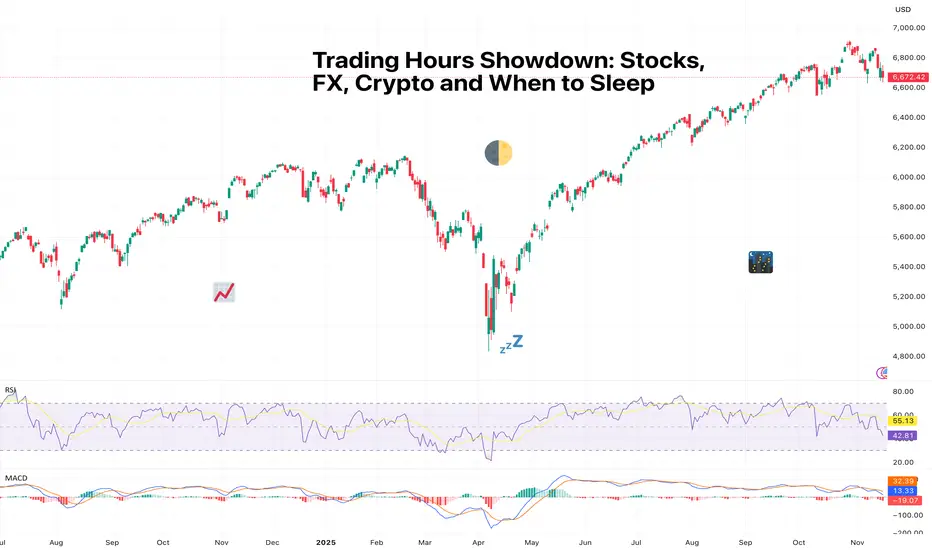
Trading Hours Showdown: Stocks, FX, Crypto and When to SleepSome markets close, some don’t, and some don’t care that you need rest.
If financial markets were people, they’d each have wildly different sleeping habits. Stocks tuck themselves in usually at 4 p.m. (that is, where they originate from), FX stays up all night but insists it’s “fine,” and crypto is that friend who messages you at 3 a.m. with a life-changing idea (and a 12% move for fun).
Understanding when each market is awake, liquid, and volatile is one of the most underrated skills a trader can have. It’s not just about timing entries; it’s about managing risk while you’re away from your devices.
Let’s break down the global sleep schedule and why your portfolio should care.
🌅 Stocks: The 9-to-5ers of the Financial World
US stocks like routine. They open at 9:30 a.m. ET, close at 4 p.m., and observe weekends and holidays like well-behaved citizens.
There’s also pre-market and after-hours trading, but liquidity dries up real fast and moves tend to be exaggerated.
Why it matters:
Limited hours = overnight gap risk
Most volume typically happens in the first and last 30 minutes
Big news after hours can cause violent opens the next day
Stops can’t protect you when price jumps over your level
Every trader eventually experiences the heartbreak of a perfect setup ruined by an overnight earnings surprise. Consider it a rite of passage.
🌍 Forex: The Market with No Bedtime
FX ( forex or foreign exchange) trades 24 hours a day, five days a week, rotating through global sessions:
Asia (Tokyo)
Europe (London)
US (New York)
That’s a 120-hour work week with no break. Think of it like a global relay race where someone is always awake and analyzing inflation differentials.
Why traders love it:
Continuous liquidity = fewer gaps
Beautiful macro-driven trends
Volatility waves follow session overlaps (London–NY especially)
But…
FX weekends could be silent killers. You’re unprotected from Friday close to Sunday open. That’s plenty of time for geopolitical headlines, surprise events, central bank drama, or a country deciding to unpeg its currency.
🔥 Crypto: The Market That Never Sleeps or Blinks
The cryptocurrency market trades 24/7/365. No days off, no weekends, no holidays, no rest. Just pure, unfiltered price action around the clock.
This sounds great until you realize you can never fully unplug. Bitcoin BITSTAMP:BTCUSD does not respect your circadian rhythm.
Why it’s unique:
No “overnight gaps” because it never closes
But liquidity gaps may appear during low-volume hours
Late-night moves can be extreme due to thin order books
Leverage unwinds can trigger liquidation cascades at 3 a.m.
Global retail participation exaggerates emotional spikes
Crypto doesn’t gap like stocks, but it drifts, snaps, and rips through levels and can make your stomach churn.
🧭 Liquidity: The Real Story Behind the Sleep Schedule
Across markets, the one concept that ties them all together is liquidity. That is, how deep the order book is and how efficiently your trades can execute.
Stocks
Thick liquidity during US hours
Thin, jumpy after-hours
Prone to large news-driven gaps
Forex
Deep liquidity almost 24 hours a day
Most volume during London–NY overlap
Macro news instantly reflected in price
Crypto
Liquidity pockets vary wildly
Exchanges differ in depth
Weekends and Asia-over-US crossovers can trigger whipsaws
😴 The Question of Sleep (And How Traders Manage It)
Traders eventually learn a few things about trading various asset classes.
If you:
Hate surprises → Avoid overnight stock positions
Love macro trends → FX is your playground
Enjoy volatility → Crypto keeps things interesting
Value sleep → Choose an asset class that aligns with your time zone and day trade it
Choosing a market to trade isn’t just about your strategy, but also about your lifestyle.
Volatility doesn’t just depend on the asset. It depends on when you’re watching.
Off to you : How do you deal with trading different assets in different time zones? Are you a niche player or a broader market maven? Share your comments below!
How to build a Healthy Trading MindsetMany traders underestimate how much psychology shapes their results. This guide outlines the foundations of a strong trading mindset that supports consistent and disciplined decision-making.
1. Understand That Emotional Discipline Is a Skill
Trading naturally triggers emotions such as fear, frustration, greed, and impatience. These reactions are not weaknesses; they are human. What separates consistent traders from inconsistent ones is their ability to recognize emotions without acting on them.
A resilient mindset comes from training, not talent.
2. Create Distance Between Yourself and Your Trades
Do not tie your self-worth to the outcome of a single position. A loss does not mean you failed, and a win does not mean you are skilled. When traders begin to link identity to results, they make impulsive decisions.
Use phrases like “this trade” instead of “my trade” to remove ownership bias.
3. Focus on Process, Not Profit
Most traders sabotage themselves by obsessing over the end result. The market does not reward effort; it rewards alignment with probability.
Instead of thinking “How much can I make?”, think “Did I execute according to my plan?”
Your trading plan should define your entries, exits, risk, and market conditions. Follow it even when it feels uncomfortable.
4. Accept Uncertainty as Part of the Game
No setup is guaranteed. Every trade, no matter how perfect, carries uncertainty. Accepting this prevents you from forcing control where none exists.
When you fully accept uncertainty, you no longer fear it.
5. Build Consistency Through Routine
A stable routine reduces mental noise. Examples include:
• Reviewing your plan before each session
• Limiting how many markets you monitor
• Taking breaks after high-stress situations
• Logging your trades with honest notes
When your routine is consistent, your decisions become consistent.
6. Use Losses as Data, Not Drama
A loss is not a personal attack from the market. It is information.
Ask: “What does this loss teach me about my system or my mindset?”
If you can extract value from losses, they become opportunities instead of obstacles.
7. Master Patience
Most trading errors come from acting too soon, not too late. Patience means waiting for your setup without deviation.
If you need to be in a trade at all times, it is no longer trading; it is compulsion.
8. Protect Your Mental Capital
Mental capital is as important as financial capital. Overtrading, revenge trading, and excessive chart time drain your cognitive energy.
Stop trading when you notice fatigue, frustration, or impulsiveness. A clear mind is an advantage.
9. Develop Long-Term Thinking
Think in terms of series, not individual outcomes. A single win or loss means little. What matters is the overall direction of your equity curve.
Professional traders think in months and years. Amateurs think in minutes.
Conclusion
A powerful trading mindset is built through consistency, self-awareness, and emotional control. By focusing on process and discipline rather than short-term results, you create a stable internal environment that supports longevity in the markets.
Mastering RSI: A Complete Guide to Momentum🔵 Mastering RSI: A Complete Guide to Momentum, Regimes, Reversals & Professional Signals
Difficulty: 🐳🐳🐳🐳🐋 (Advanced)
This article goes far beyond the basic idea of “RSI = overbought/oversold.” If you want to truly master RSI as a momentum gauge, trend filter, reversal tool, and structure confirmation model, this guide is for you.
🔵 WHY MOST TRADERS MISUSE RSI
Most traders use RSI in the simplest way:
RSI above 70 = sell
RSI below 30 = buy
This leads to shorting strong trends and catching falling knives.
RSI is not a reversal button. RSI is a momentum translator.
To master RSI, you must understand:
Trend regimes
Momentum pressure
Acceleration and deceleration
Failure swings
Divergences
Trend vs range behavior
Multi-timeframe alignment
Structure confirmation
RSI shows the strength behind price, not just extremes.
🔵 1. RSI TREND REGIMES (CORE FOUNDATION)
RSI moves in predictable zones depending on the type of market environment.
Bullish RSI Regime
RSI holds between 40 and 80
Pullbacks bottom around 40–50
Breaks above 60 show trend acceleration
Bearish RSI Regime
RSI holds between 20 and 60
Pullback tops form around 50–60
Breaks below 40 confirm bearish dominance
These regimes tell you who controls the market before you even look at candles.
🔵 2. MOMENTUM PRESSURE (RSI AS A SPEEDOMETER)
RSI measures the speed and pressure of price movement.
Rising RSI with rising price = trend acceleration
Falling RSI with rising price = momentum weakening
Rising RSI with falling price = early strength
Falling RSI with falling price = continuation pressure
This is not divergence. It is momentum pressure, the earliest sign of trend shift.
🔵 3. FAILURE SWINGS (THE MOST RELIABLE RSI REVERSAL SIGNAL)
Failure swings are powerful because they show internal momentum breaking before price reacts.
Bullish Failure Swing
RSI makes a low
RSI rallies
RSI dips again but stays above previous low
RSI breaks the previous high
Bearish Failure Swing
RSI makes a high
RSI pulls back
RSI rallies but fails to break the previous high
RSI breaks the previous low
Failure swings often appear at trend tops and bottoms before candles reveal anything.
🔵 4. DIVERGENCES (REGULAR AND HIDDEN)
Regular Divergence: Reversal Clue
Bullish: price lower low, RSI higher low
Bearish: price higher high, RSI lower high
Hidden Divergence: Trend Continuation
Bullish hidden: price higher low, RSI lower low
Bearish hidden: price lower high, RSI higher high
Hidden divergence is more powerful than regular because it confirms trend continuation.
🔵 5. RANGE RSI VS TREND RSI
RSI behaves very differently in ranges versus trends.
Range Environment
RSI oscillates between 30 and 70
Reversals at extremes have high accuracy
RSI 50 is the equilibrium
Trend Environment
RSI stays above 50 in bullish trends
RSI stays below 50 in bearish trends
30 and 70 extremes lose meaning
Always identify environment first. RSI signals change depending on regime.
🔵 6. RSI AS A STRUCTURE FILTER
RSI combined with structure improves trade selection dramatically.
Price makes higher highs + RSI rising = healthy trend
Price makes higher highs + RSI flat = weak breakout
Price makes higher highs + RSI dropping = exhaustion
Support retest + RSI 40–50 = strong continuation potential
Most false breakouts are avoided simply by checking RSI pressure.
🔵 7. MULTI-TIMEFRAME RSI ALIGNMENT
Use higher timeframe RSI to validate lower timeframe setups.
HTF RSI bullish + LTF RSI pullback = high-quality entry
HTF RSI bearish + LTF RSI bounce = premium short area
HTF RSI crossing 50 = long-term regime shift
This is one of the most powerful RSI confluences.
🔵 EXAMPLE TRADING FRAMEWORK
Bullish Setup Checklist
RSI in bullish regime (above 50)
Pullback into 40–50 zone
Hidden bullish divergence or failure swing
Structure forms a higher low
Bearish Setup Checklist
RSI in bearish regime
Rejection from 50–60 zone
Hidden bearish divergence or failure swing
Structure forms a lower high
🔵 COMMON RSI MISTAKES
Trading RSI extremes without trend context
Ignoring RSI regimes
Entering on regular divergences in strong trends
Not using RSI midline (50) as a regime filter
Relying only on overbought/oversold signals
🔵 CONCLUSION
RSI is one of the most powerful indicators when used correctly. It provides a complete framework for:
Reading trend strength
Tracking momentum pressure
Identifying early reversals
Trading continuation setups
Filtering breakout strength
Aligning multi-timeframe bias
Master RSI, and you gain a clearer view of momentum than most traders ever experience.
How do you use RSI? Do you prefer divergences, trend zones, or failure swings? Share your approach below!

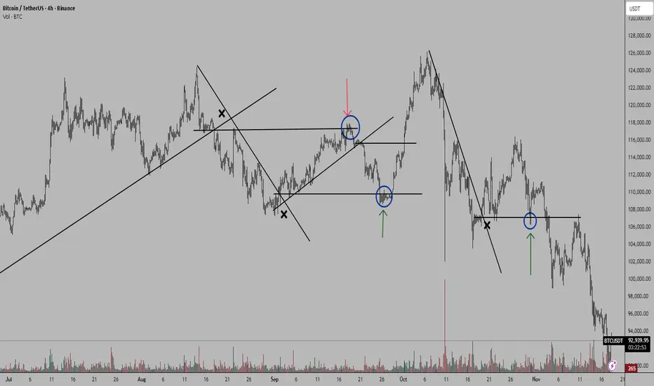
Crypto Cycle: The Arrogance and The Irony — A Must ReadThe Cycle That Changed Everything
This cycle — which really started in October 2023 — broke every pattern from previous crypto bull runs.
Crypto was created as a rebellion:
Freedom from banks.
An anti-system technology.
Privacy.
Self-sovereignty.
A way for normal people to create wealth without permission.
And yet… somehow the exact people crypto was trying to escape have taken control of it.
Retail investors used to love the idea of owning their finances. No more banks telling them what to do. No more gatekeepers.
Until they arrived.
1 — The Arrogance
The rich run the world — that’s nothing new.
But crypto annoyed them. A lot.
Because crypto allowed ordinary people to do what Wall Street hates most:
Make money without giving the rich a cut.
So what did institutions do?
Simple:
“If you can’t kill it… own it.”
They stopped fighting crypto, took over the market, bought the exchanges, injected billions, partnered with the stablecoin printers, and unleashed industrial-scale manipulation.
The old days of making x10 or x100 on leverage?
Gone.
Retail got liquidated again… and again… and again.
Bitcoin pumped 3 times by billionaires (just look at the three green boxes on the chart).
Retail got excited — then destroyed.
Rinse and repeat.
Eventually, retail gave up.
They moved into gold, silver, or even plain USD — just to stop losing money.
Meanwhile institutions kept pumping Bitcoin and Ethereum artificially, hoping to lure back fresh meat…
but nobody came.
2 — The Irony
Then came October 11, 2025 — the day the curtain fell.
In a dry, illiquid market, Binance did their usual liquidation-hunting game, backed by newly-printed billions from Tether:
2 billion minted one day, 2 billion the next.
They pushed Bitcoin to $126,000.
Then the crash hit.
They chased longs so hard that, in a market with no liquidity, the entire altcoin market collapsed.
Some coins literally went to zero.
Binance had to halt trading.
The liquidation chain couldn’t be stopped.
Some market makers lost everything.
And now they’re furious.
Binance got exposed.
The pump-and-dump machine is broken.
And if they continue, they risk criminal investigations and lawsuits from every direction.
Suddenly BlackRock, Saylor, and friends had a problem:
Their favorite manipulation partner was knocked out.
And that’s when reality hit:
Institutions had pushed Bitcoin so high — without retail — that they found themselves holding billions in assets…
…with nobody left to buy their bags.
Old-time Bitcoin holders realized BTC was compromised and began to sell.
Bitcoin maxis rekt the institutions.
The billionaires who bought at $120k got destroyed by the exact people they planned to destroy.
Karma doesn’t miss.
Even Eric Trump started selling — too late.
Bitcoin fell under $89k, and there were no buyers left.
3 — The Lesson
Institutions need to understand one thing:
Crypto is not for institutions.
The tech? Sure.
The coins? No.
Crypto without retail is like a vampire trying to drink its own blood.
Pointless and self-destructive.
And retail won’t return for “fractional Trump coin” or corporate-approved BTC.
Retail wants:
x10, x100, x1000.
That means one thing:
ALTSEASON.
If institutions want liquidity to exit, they must engineer an altseason and share some profits.
Because without retail, they’re stuck in their expensive echo chamber holding overpriced bags that nobody wants.
And if they do create an altseason?
Retail will dump on them harder than ever — watching TradingView and influencers, selling every rally right back into the institutions’ faces.
Wall Street, stick to Wall Street.
Leave crypto to the crypto degenerates.
It’s a wild jungle, and you were never prepared.
#CryptoCycle #BitcoinCrash #AltseasonWhen #CryptoHumor #MarketManipulation #InstitutionsRekt #BinanceDrama #RetailVsWhales #CryptoReality #KarmaInCrypto #CryptoStory #PattayaCryptoDegens

Crypto Market Trends (Bitcoin, Ethereum, Stablecoins)1. Bitcoin Trends
Bitcoin (BTC), the world’s first and most widely recognized cryptocurrency, remains the benchmark for the entire digital asset market. Several recent trends shape its behavior:
A. Institutional Adoption Accelerates
Institutional involvement has grown consistently, driven by exchange-traded products, corporate investments, and hedge funds using Bitcoin as an alternative asset. The approval of spot Bitcoin ETFs in major economies (primarily the US and a growing list of other countries) has created new channels of capital inflow. These funds have attracted billions of dollars in assets under management, making Bitcoin more accessible to traditional investors.
B. Bitcoin as a Macro-Driven Asset
Bitcoin is increasingly treated like a risk-on macro asset influenced by:
Global interest rates
Inflation expectations
U.S. Federal Reserve monetary policy
Liquidity cycles
During periods of rate cuts or economic uncertainty, Bitcoin often attracts attention as “digital gold” or a hedge against currency debasement. Conversely, when rates rise and liquidity tightens, BTC experiences downward pressure.
C. Halving Cycles and Supply Shock
Bitcoin operates on a fixed supply of 21 million coins, with block rewards halving every four years. Each halving reduces the rate of new BTC entering the market. Historically, these events lead to:
Reduced selling pressure from miners
Increased scarcity-driven demand
Potential long-term bullish cycles
Even after each halving, the narrative of Bitcoin as a scarce, deflationary asset strengthens.
D. Growing Role in Global Money Transfers
Bitcoin usage in cross-border payments has surged due to:
Lower transaction fees via the Lightning Network
Faster settlement times
Limited dependency on traditional banking systems
This trend is especially prominent in countries facing currency crisis, inflation, or capital controls.
E. Market Maturity and Reduced Volatility
Compared to earlier years, Bitcoin’s volatility has begun to moderate as liquidity increases and institutional participation grows. This does not eliminate major price swings, but BTC is gradually moving toward being a more established asset class.
2. Ethereum Trends
Ethereum (ETH) dominates the smart contract and decentralized application ecosystem. It serves as the backbone for decentralized finance (DeFi), NFTs, tokenization, and much more. Ethereum trends include:
A. Transition to Proof of Stake (PoS)
The successful transition from Proof of Work (PoW) to Proof of Stake (PoS)—known as the Merge—has permanently shifted Ethereum’s energy consumption and security model. The PoS upgrade has:
Reduced energy usage by ~99%
Made staking a core yield-generating activity
Enhanced network security through validator decentralization
ETH staking continues to grow, locking a significant portion of supply away from active circulation.
B. Surge in Ethereum Layer-2 Ecosystems
Ethereum’s scalability challenges led to the rise of Layer-2 chains like:
Arbitrum
Optimism
Base
zkSync
StarkNet
These chains:
Reduce transaction fees
Increase processing speed
Expand Ethereum’s usability for retail users
The long-term trend is toward Ethereum becoming the settlement layer while L2s handle high-volume activity.
C. Tokenization of Real-World Assets (RWA)
One of the fastest-growing sectors on Ethereum is asset tokenization. Institutions are issuing blockchain-based representations of:
Government bonds
Real estate
Corporate debt
Money-market funds
Tokenized U.S. Treasury products on Ethereum have grown rapidly, showing real institutional use beyond speculation.
D. Ethereum as the Base Layer for DeFi
Even after market cycles and volatility, Ethereum remains the dominant chain for:
Lending protocols (Aave, Compound)
Decentralized exchanges (Uniswap, Curve)
Price oracles (Chainlink)
Yield staking
Total Value Locked (TVL) tends to rise and fall with overall market sentiment, but Ethereum consistently holds the largest share.
E. Shift Toward Deflationary Supply
After EIP-1559 introduced base fee burning, Ethereum sometimes becomes deflationary, meaning more ETH is burned than issued—especially during periods of high network activity. This creates a long-term bullish supply dynamic similar to Bitcoin’s scarcity.
3. Stablecoin Trends
Stablecoins are the foundation of global crypto liquidity. They provide stability, enable global transactions, and serve as a bridge between traditional finance (TradFi) and decentralised finance (DeFi).
A. Rapid Growth in Market Capitalization
Stablecoins like USDT, USDC, and emerging decentralized alternatives have seen strong growth. They are increasingly used for:
Trading pairs on crypto exchanges
Remittances
Yield generation
On-chain settlement
DeFi collateral
USDT continues to dominate due to its wide availability and high adoption in cross-border markets.
B. Regulatory Tightening and Transparency
Governments worldwide are enforcing stricter oversight of stablecoins. The aim is to ensure:
1:1 reserve backing
Independent audits
Stronger disclosure requirements
These regulations help institutional adoption and reduce risks associated with opaque issuers.
C. Rise of On-chain Payments
Stablecoins are rapidly emerging as a global payments infrastructure. Businesses and fintech companies increasingly use stablecoins for:
Payroll
B2B transfers
E-commerce
Cross-border settlements
Their speed, low cost, and 24/7 availability make them an attractive alternative to SWIFT.
D. Competition from CBDCs
Central banks globally are experimenting with Central Bank Digital Currencies (CBDCs). Although CBDCs will coexist with stablecoins, they may compete in retail and wholesale payments. Stablecoins, however, retain the advantage of flexibility, programmability, and cross-chain mobility.
E. Decentralized Stablecoins Return
Decentralized options like DAI and FRAX are evolving to become more resilient. The trend is toward:
Overcollateralized models
Multi-asset backing
Algorithmic governance with strong safety features
This helps reduce dependence on centralized issuers.
4. Combined Crypto Market Themes
A. Institutionalization of Crypto
Bitcoin, Ethereum, and stablecoins together form the backbone for large institutions entering the market. Their maturity and regulatory clarity provide confidence for long-term investment.
B. Integration with Traditional Finance
Crypto is increasingly merging with traditional financial rails:
Tokenized stocks
Tokenized treasury bonds
Crypto payment cards
Stablecoin-powered banking services
C. Market Cycles Driven by Liquidity
Crypto markets remain heavily influenced by global liquidity. When monetary conditions ease, capital flows into BTC and ETH first, then spreads to altcoins.
D. On-Chain User Growth
Wallet creation, transaction counts, staking participation, and L2 adoption are rising steadily. Crypto is shifting from speculation to real-world usage.
Conclusion
Bitcoin, Ethereum, and stablecoins represent the three fundamental pillars of the modern cryptocurrency ecosystem. Bitcoin leads as a global digital store of value, Ethereum powers decentralized applications and financial innovation, while stablecoins act as the liquidity engine for global on-chain activity. Together, these sectors continue to grow due to institutional adoption, technological advancements, and increased global demand for decentralized alternatives to traditional financial systems. As regulatory clarity emerges and more real-world uses develop, these assets are positioned to drive the next phase of crypto market expansion.
Artificial Intelligence & Tech Stocks Rally1. The Rise of AI as an Economic Catalyst
AI has shifted from being a futuristic concept to a real-world productivity enhancer. It now influences every major industry: financial services, healthcare, manufacturing, retail, cybersecurity, logistics, and more. Technologies such as deep learning, natural language processing, and autonomous systems have prompted companies worldwide to accelerate their digital transformation.
The introduction of large language models (LLMs), AI chips, robotics, and automation has created a new economic cycle driven by data, computing power, and algorithmic intelligence. As a result, companies directly involved in AI development—along with those supplying the hardware and cloud platforms—have become market favorites.
Investors increasingly view AI as the next “industrial revolution” capable of reshaping global productivity, profitability, and innovation. This belief has driven massive capital inflows into tech stocks, especially those perceived as leaders in AI research and commercialization.
2. Key Drivers Behind the AI-Fueled Tech Rally
A. Explosive Growth of Generative AI
The launch of advanced generative AI systems dramatically accelerated interest in AI stocks. Major companies quickly integrated generative AI into search engines, productivity tools, customer support, and software development workflows. This rapid adoption strengthened the revenue outlook for tech giants and reinforced investor confidence.
B. Demand for High-Performance Computing & AI Chips
Semiconductor companies, particularly those producing AI GPUs and specialized accelerators, have emerged as the backbone of the AI revolution. The massive need for computational power has pushed chip manufacturers to record valuations. Cloud service providers and hyperscale data centers are investing billions to upgrade their infrastructure to handle AI workloads.
C. Cloud Expansion & Software AI Integration
Tech firms integrating AI into their existing cloud and software offerings have seen rising subscription revenue and improved customer retention. The “AI upgrade cycle”—where businesses adopt AI features as part of cloud services—has enhanced long-term earnings visibility for cloud companies.
D. Automation & Productivity Gains
AI-driven automation is helping businesses improve productivity while reducing costs. Companies that demonstrate measurable efficiency gains from AI adoption are rewarded by investors, who view this as margin-expansion potential. As firms show better earnings due to AI-enabled efficiencies, market optimism increases.
E. Global Government Support
Governments worldwide are prioritizing AI policy, infrastructure, and innovation funding. This includes national AI strategies, incentives for semiconductor manufacturing, and investment in digital public infrastructure. These initiatives create favorable environments for AI-driven business growth, further strengthening investor sentiment.
3. Major Sectors Benefiting from the AI Rally
1. Semiconductor & Chip Manufacturing
AI requires enormous computing power, leading to unprecedented demand for GPUs, neural processing units (NPUs), and specialized chips. Semiconductor companies have seen massive revenue growth due to AI training and inference workloads.
2. Cloud Computing Platforms
AWS, Microsoft Azure, Google Cloud, and others are increasingly viewed as the “AI backbone” because they host AI models and provide infrastructure. Cloud giants benefit from scalable subscription revenue and enterprise AI spending.
3. Software as a Service (SaaS)
SaaS companies integrating AI into CRM, automation, analytics, and productivity tools are experiencing an upgrade cycle. New AI features allow them to charge premium subscription fees, boosting profitability.
4. Cybersecurity
AI-powered cybersecurity systems detect threats faster and manage huge volumes of data. With rising cybercrime, demand for AI-based security tools continues to expand.
5. Robotics & Automation
AI is powering industrial robotics, warehouse automation, and autonomous machinery. The increased demand for efficiency in logistics and manufacturing fuels revenue growth for automation firms.
6. Consumer Technology
AI is enhancing smartphones, smart home systems, wearables, and personal digital assistants. Tech companies adding AI capabilities have seen surging demand for next-generation devices.
4. Why Investors Are Bullish on AI's Long-Term Outlook
A. Multi-Trillion Dollar Market Potential
AI’s total addressable market (TAM) is expected to surpass trillions of dollars over the next decade. Analysts predict long-term growth across nearly every industry, making AI one of the largest commercial opportunities in history.
B. Continuous Innovation & Rapid Deployment
AI models and systems improve continuously. Every new innovation—smarter models, faster chips, more efficient algorithms—creates new commercial opportunities. This rapid pace of change fuels sustained investor enthusiasm.
C. Enterprise Adoption at Massive Scale
Companies across sectors are integrating AI into operations, decision-making, and customer experience. Enterprise adoption is one of the biggest drivers of long-term revenue growth for AI suppliers and service providers.
D. Network Effects & Data Advantages
Companies with massive data pools, extensive user bases, and strong computational capacity benefit from network effects. This creates “winner-take-most” dynamics favoring tech giants—which attract substantial investor capital.
5. Risks & Challenges to the AI Tech Rally
While the AI-driven rally is strong, it is not without risks:
1. Overvaluation Concerns
Some tech stocks have reached extremely high valuations. If earnings growth fails to match expectations, corrections may occur.
2. Supply Chain Constraints
AI hardware requires complex semiconductor supply chains. Shortages in advanced chips could impact production and revenue.
3. Regulatory & Ethical Uncertainty
Governments are increasing oversight over AI data use, privacy, and safety. Regulatory risks can affect growth prospects.
4. High Capital Expenditure
AI infrastructure—data centers, chips, cloud systems—is extremely expensive. Some companies may face profitability pressures due to high capex.
5. Competitive Intensity
AI markets are highly competitive. New entrants, rapid innovations, or pricing pressures could disrupt market leaders.
6. Future Outlook of AI & Tech Stocks
The long-term outlook for AI and tech remains highly positive. Over the next decade, AI is expected to shape global economic growth, productivity, and technological innovation. Key trends include:
Expansion of generative AI across enterprise workflows
Surge in demand for AI chips, data centers, and cloud computing
Growing adoption in healthcare, finance, logistics, education, and retail
AI-powered robotics reshaping manufacturing
Increased global investment in digital and computational infrastructure
Despite market volatility or occasional corrections, AI’s economic impact is expected to grow significantly, making AI and tech stocks central to modern global portfolios.

Equity Market Indices (S&P 500, Nasdaq, DAX, Nikkei)1. S&P 500 Index — The Global Benchmark
The Standard & Poor’s 500 Index, commonly known as the S&P 500, is one of the world’s most followed equity indices. It tracks 500 of the largest publicly listed companies in the United States. Unlike the Dow Jones Industrial Average, which uses price weighting, the S&P 500 uses free-float market capitalization weighting, making it a more accurate representation of the U.S. equity market.
Structure and Components
The index spans all major U.S. sectors, including technology, financials, healthcare, consumer discretionary, and energy. Mega-cap companies like Apple, Microsoft, Amazon, and Alphabet often dominate the index due to their large market capitalizations.
Economic Significance
The S&P 500 accounts for over 80% of U.S. total market value, making it a barometer for overall U.S. corporate health. Movements in the index reflect:
Corporate earnings trends
Investor sentiment
Monetary policy expectations
Global macroeconomic factors
Investment and Trading Use
Investors use the S&P 500 for:
Benchmarking fund performance
ETF and index fund investing (e.g., SPY, VOO)
Futures and options trading
Analysts often interpret a rising S&P 500 as a sign of economic expansion, while prolonged declines may indicate recession concerns.
2. Nasdaq Composite & Nasdaq-100 — Tech-Heavy Growth Indicators
The Nasdaq Composite is one of the most technology-heavy indices in the world, tracking over 3,000 stocks listed on the Nasdaq exchange. The more popular trading index, however, is the Nasdaq-100, which includes the top 100 non-financial companies on Nasdaq.
Technology Dominance
The Nasdaq is dominated by:
Technology
Internet services
Biotechnology
Semiconductor companies
Major names include Apple, Microsoft, Nvidia, Meta, and Tesla.
Characteristics and Sensitivity
Because it is tech-heavy, the Nasdaq tends to be:
More volatile than the S&P 500
Highly sensitive to interest rate changes
Influenced strongly by innovation trends, earnings expectations, and regulatory actions
Growth stocks, which dominate the Nasdaq, typically outperform during low-interest-rate environments when borrowing is cheaper and future earnings are more valuable.
Use for Traders
Traders often use the Nasdaq as a sentiment gauge for:
Tech sector strength
Risk appetite in markets
Momentum-driven trading strategies
Nasdaq futures (NQ) and ETFs like QQQ are among the most actively traded instruments globally.
3. DAX (Germany) — Europe’s Industrial Power Index
The DAX (Deutscher Aktienindex) is Germany’s leading stock index, representing 40 blue-chip companies listed on the Frankfurt Stock Exchange. Unlike other indices, the DAX is a performance index, meaning dividends are reinvested, resulting in slightly higher long-term returns.
Composition
The DAX includes major industrial, automotive, chemical, and financial giants such as:
Siemens
Volkswagen
Mercedes-Benz
Bayer
Allianz
SAP
Role in Europe
Germany is Europe’s largest economy, so the DAX essentially acts as a proxy for the health of the Eurozone economy. It reflects:
Manufacturing output
Export competitiveness
Global demand for automobiles and engineering
Euro currency movements
Key Drivers
The DAX is influenced by:
European Central Bank (ECB) policies
Eurozone inflation and GDP
Geopolitical relations with the U.S. & China
Energy prices (Europe is energy-dependent)
During periods of higher global industrial activity, the DAX typically performs strongly due to Germany’s export-led economy.
4. Nikkei 225 — Japan’s Economic Indicator
The Nikkei 225, Japan’s best-known stock index, tracks 225 top companies on the Tokyo Stock Exchange. Unlike most major indices, the Nikkei is price-weighted, similar to the Dow Jones, meaning higher-priced stocks have greater influence regardless of company size.
Sector Mix
Japan’s market includes a mix of:
Automotive companies (Toyota, Honda, Nissan)
Consumer electronics (Sony, Panasonic)
Industrial manufacturers (Fanuc, Hitachi)
Financial institutions
Economic Importance
The Nikkei reflects Japan’s:
Export competitiveness (especially to the U.S. and China)
Yen strength or weakness
Domestic consumption trends
Bank of Japan (BOJ) monetary policy
Japan's prolonged period of low interest rates and deflation has historically shaped the Nikkei’s long-term performance.
Yen Relationship
The Nikkei tends to rise when the Japanese yen weakens, because a weaker yen boosts export revenues. It often behaves inversely to USD/JPY currency movements.
5. How Traders Use These Indices
Market Sentiment Indicators
Each index provides insight into different segments:
S&P 500: overall U.S. economy
Nasdaq: tech and growth sentiment
DAX: European industrial strength
Nikkei: Asian economic trends
Sector Rotation
Investors analyze relative performance to gauge:
Growth vs. value cycles
Domestic vs. international capital flows
Risk-on vs. risk-off behavior
Hedging & Diversification
Indices are widely used for:
Portfolio diversification
Hedging through futures/options
ETF investing across regions
Correlation Behavior
S&P 500 and Nasdaq have high correlation
DAX moves closely with global manufacturing trends
Nikkei correlates strongly with currency markets
Understanding these correlations helps global traders manage risk and time their entries.
6. Global Impact of Index Movements
Because these are major world indices, movements can influence:
Commodity prices (oil, gold)
Currency valuations (USD, EUR, JPY)
Bond markets
Emerging market flows
For example:
A strong S&P 500 often attracts global capital into the U.S.
Weak DAX performance can signal European recession fears
A rising Nikkei can lift Asian equity sentiment
Conclusion
Equity market indices like the S&P 500, Nasdaq, DAX, and Nikkei 225 are more than just collections of stock prices. They are critical indicators of economic health, investor behavior, and global financial stability. Each index reflects the structure of its economy—U.S. technology leadership for Nasdaq, diversified large caps for the S&P 500, industrial might for the DAX, and export-driven growth for the Nikkei. Together, they form the backbone of global equity analysis and remain essential tools for traders, investors, and policymakers worldwide.

Gold & Safe-Haven Asset Trading1. Why Gold Is Considered a Safe-Haven Asset
Gold is perceived as a safe-haven for several reasons:
1.1 Intrinsic Value
Gold is a physical asset with limited supply. It cannot be printed like fiat currency, and mining output grows slowly over time. This scarcity gives gold long-term value stability.
1.2 Universal Acceptance
Gold is accepted globally as a store of value by governments, central banks, banks, institutions, and retail investors. It is one of the few assets that retain value regardless of the political or economic system in place.
1.3 Hedge Against Inflation & Currency Depreciation
When inflation rises or a currency weakens—especially the USD—gold prices tend to increase. This is because investors shift capital into assets that preserve purchasing power.
1.4 Geopolitical Crisis Shield
During wars, conflicts, sanctions, or major political uncertainty, gold attracts strong demand. Institutions rotate out of risk assets like equities and into safer stores of value.
1.5 Negative Real-Yield Environment
When real interest rates (interest rate minus inflation) fall or turn negative, the opportunity cost of holding non-yielding gold decreases, making it more attractive.
2. What Are Safe-Haven Assets?
Safe-haven assets are those that retain or increase value during times of market volatility, economic crisis, or geopolitical stress. The key safe-haven categories include:
Gold
US Dollar (USD)
US Treasury bonds
Japanese Yen (JPY)
Swiss Franc (CHF)
Silver and other precious metals
Sometimes: utilities, consumer staples, defensive stocks
Gold remains the most universal and liquid among them.
3. Key Drivers of Gold Prices
To trade gold effectively, traders must understand the main price drivers:
3.1 US Dollar Index (DXY)
Gold is priced in USD globally.
A stronger USD → gold becomes expensive for holders of other currencies → gold falls
A weaker USD → gold becomes cheaper globally → gold rises
This inverse relationship is one of the strongest correlations in global markets.
3.2 Interest Rates (Especially US Treasury Yields)
Gold does not pay interest. When yields rise, gold becomes less attractive.
Rising yields → bearish for gold
Falling yields → bullish for gold
Real yields matter more than nominal yields.
3.3 Inflation
Gold is a traditional inflation hedge.
Higher inflation → gold demand increases → gold prices rise
Low/deflation → gold weakens
3.4 Geopolitical & Financial Risks
Gold spikes during:
wars
banking system stress
sovereign debt crises
market meltdowns
oil price shocks
trade wars
currency crises
Gold thrives when uncertainty rises.
3.5 Central Bank Gold Purchases
Many central banks buy gold to diversify reserves away from the USD.
Large purchases by China, India, Russia, and emerging markets support gold prices.
3.6 ETF Flows
Gold-backed ETFs (like SPDR Gold Trust – GLD) influence prices through physical purchasing.
4. Gold Trading Instruments
4.1 Spot Gold (XAU/USD)
The most traded instrument in gold markets.
XAU/USD represents gold priced in U.S. dollars.
4.2 Gold Futures (COMEX)
Highly liquid and used by institutional investors and hedgers.
4.3 Gold ETFs (GLD, IAU)
Useful for passive investors or those who want gold exposure without physical storage.
4.4 Gold Mining Stocks
Companies like Barrick Gold, Newmont etc.
Mining stocks are leveraged plays on gold prices.
4.5 Physical Gold (Bars, Coins)
Used mostly for long-term wealth preservation.
5. Safe-Haven Flow Dynamics
Understanding how capital flows during crises is key.
5.1 Risk-Off Environment
When market fear rises:
Equities fall
Bond yields drop
USD and gold rise
Gold attracts capital as a non-correlated asset.
5.2 Risk-On Environment
When markets recover:
Equities rise
USD strengthens
Gold often consolidates or corrects
Safe-haven demand decreases.
6. Trading Strategies for Gold & Safe-Haven Assets
6.1 Trend Following Strategy
Since gold often moves in strong directional trends:
Use moving averages (50/200 EMA)
Buy when price is above key MAs and forming higher highs
Sell when price breaks below MAs with strong volume
6.2 Breakout Strategy
Gold reacts strongly to breakouts from:
price consolidation zones
triangle patterns
wedge patterns
horizontal ranges
A breakout with high volume can signal a strong move.
6.3 Mean Reversion (Contrarian) Strategy
Gold frequently retraces after sharp moves.
Indicators:
RSI (overbought/oversold)
Bollinger bands
Price divergence
Use cautiously during trending markets.
6.4 Macro-Based Trading
Use fundamental triggers:
Fed interest rate decisions
CPI inflation releases
NFP jobs report
Geopolitical events
Central bank speeches
These can cause rapid volatility in gold.
6.5 Safe-Haven Correlation Trading
You can trade gold relative to:
DXY movements
US 10-year yield changes
JPY or CHF moves
VIX index spikes
When volatility rises, gold usually rallies.
7. Gold in Portfolio Diversification
Gold is one of the best hedges against:
inflation
currency weakness
economic slowdowns
stock market crashes
Historically, gold has low correlation with equities, making it ideal for diversification.
Portfolio strategies:
5–10% gold allocation for stability
15–20% during high inflation periods
Use gold to hedge global macro risks
8. Risks in Gold Trading
Despite being a safe-haven, gold trading carries risks:
8.1 High Volatility
Gold can move sharply around:
CPI
NFP
Fed meetings
geopolitical headlines
8.2 Interest Rate Shocks
An unexpected spike in yields can cause large downside in gold.
8.3 USD Strength
A strong, sudden USD rally can drag gold lower.
8.4 False Breakouts
Gold sees many fake breakouts due to liquidity-driven algorithmic trading.
8.5 Over-leveraging
Leverage in futures or CFDs can magnify losses during volatile phases.
9. Long-Term Outlook for Gold
Over decades, gold generally trends upward due to:
global inflation
rising debt levels
currency debasement
central bank gold accumulation
geopolitical risks
The long-term picture remains bullish, but short-term volatility is normal.
Conclusion
Gold and other safe-haven assets play a critical role in global financial markets, serving as stabilizers during periods of uncertainty and volatility. Gold remains the most trusted safe-haven due to its intrinsic value, global acceptance, and strong historical performance during crises. Understanding the correlations between gold, interest rates, USD, inflation, and market sentiment enables traders to anticipate market movements and trade profitably. Whether using technical setups, macro analysis, or multi-asset safe-haven flows, gold trading offers opportunities for both short-term traders and long-term investors. However, managing risk, avoiding over-leverage, and monitoring global macro signals are essential for success in gold markets.
Crude Oil Market (WTI, Brent) & OPEC+ Decisions1. Understanding WTI and Brent Crude
WTI Crude Oil
West Texas Intermediate (WTI) is a high-quality, light, and sweet crude oil primarily sourced from fields in the United States, especially Texas. Its low sulfur content makes it easier to refine into gasoline and diesel, which are in high demand in the North American market. WTI is traded on the New York Mercantile Exchange (NYMEX) and considered a benchmark for U.S. crude prices.
Brent Crude Oil
Brent is sourced from oil fields in the North Sea, spanning the UK and Norway. It is slightly heavier than WTI but still considered a light, sweet crude. Brent is traded on the Intercontinental Exchange (ICE) and acts as the global benchmark for two-thirds of internationally traded crude oil.
Why Two Benchmarks?
The existence of both benchmarks reflects regional differences in production, shipping costs, refining requirements, and market access. Generally:
WTI represents U.S. supply-demand dynamics.
Brent reflects international conditions across Europe, Asia, and Africa.
The price spread between the two (WTI–Brent spread) often indicates logistical constraints, geopolitical tensions, or shifts in global demand.
2. Factors Influencing Crude Oil Prices
Crude oil markets are volatile due to the interplay of multiple economic, geopolitical, and market-driven factors.
a. Global Supply & Demand
Oil demand is affected by:
Economic growth rates
Industrial output
Transportation needs
Seasonal factors (winter heating demand, summer driving season)
Supply depends on:
Production levels in OPEC and non-OPEC countries
U.S. shale output
Production outages or upgrades
Infrastructure constraints
b. Geopolitical Events
Conflicts in the Middle East, sanctions on major producers like Iran, instability in Venezuela, and maritime disruptions (e.g., Strait of Hormuz tensions) significantly move oil prices.
c. Currency Movements
Oil is priced in U.S. dollars.
When the USD strengthens, oil becomes expensive for foreign buyers → demand decreases → prices fall.
When the USD weakens, oil prices tend to rise.
d. Inventories & Storage
Weekly U.S. crude inventory data, especially from the EIA (Energy Information Administration), provides insights into near-term supply-demand balances.
e. Energy Transition Policies
Shift toward renewable energy, environmental policies, and long-term decarbonization targets influence investment, production, and expectations of future oil use.
3. Role of OPEC and OPEC+
What is OPEC?
The Organization of the Petroleum Exporting Countries (OPEC) was founded in 1960 to coordinate and unify petroleum policies of major producing countries. Key members include Saudi Arabia, Iraq, Iran, Kuwait, and UAE.
OPEC+ Formation
In 2016, OPEC expanded to include major non-OPEC producers such as Russia, Mexico, Kazakhstan, and others, forming OPEC+.
This group controls around 40% of global oil production and 80% of known reserves, making their decisions highly influential.
4. OPEC+ Production Decisions
a. Production Cuts
When demand falls (e.g., during pandemics or recessions), OPEC+ often cuts production to support prices.
Cuts reduce global supply → tighter market → higher prices.
b. Production Increases
During times of strong demand, OPEC+ increases output to maintain market stability.
Higher supply → pressure on prices → prevents overheating of global inflation.
c. Voluntary vs. Mandated Cuts
Sometimes individual countries choose voluntary cuts to stabilize the market.
Saudi Arabia often leads with additional voluntary cuts beyond the group agreement.
5. How OPEC+ Decisions Influence WTI and Brent
Market Expectations
Before meetings, traders speculate on whether OPEC+ will:
Cut supply
Maintain quotas
Increase production
Even rumors can create dramatic price swings.
Outcomes of Meetings
A formal announcement of cuts usually triggers:
Brent prices increasing more sharply, as it is more globally sensitive
WTI moving upward, though influenced by U.S. shale reactions
On the contrary, increases in output often lead to a pullback in both benchmarks.
Long-term Impact
Persistent cuts support a long-term bullish trend.
Persistent increases (or cheating on quotas by some members) lead to bearishness.
6. U.S. Shale Oil and the WTI–Brent Spread
One of the biggest changes in oil markets over the past decade is the rise of U.S. shale production.
Shale oil is flexible and responds quickly to price changes:
When prices rise → shale producers increase drilling
When prices fall → production slows
Because shale is mostly priced off WTI, higher U.S. output often widens the WTI–Brent spread.
Logistics Constraints
Pipeline bottlenecks in the U.S. midcontinent region can cause WTI prices to fall below Brent due to oversupply.
7. The Financialization of Oil Markets
Crude oil is not just a physical commodity—it's also a major financial asset.
Investors trade oil futures, options, ETFs, and swaps, influencing price movements.
Key players include:
Hedge funds
Banks
Producers hedging future output
Airlines hedging jet fuel costs
This financial activity creates liquidity but also increases volatility.
8. OPEC+, Price Stability, and Global Economics
Inflation Management
Crude oil is a major driver of fuel prices, transportation costs, and overall inflation.
Sharp increases in oil prices often:
Push inflation higher
Increase the chances of central bank rate hikes
Slow down economic growth
OPEC+ often aims to maintain price ranges that balance producer revenues with global economic stability.
Revenue Dependence
Many OPEC+ members rely heavily on oil revenue to fund government budgets.
Low prices strain fiscal systems; high prices improve surpluses.
9. Future of Crude Oil Markets
Short to Medium Term
Demand is expected to remain strong in developing economies.
Geopolitical risks will continue to play a major role in volatility.
Long Term
Energy transition policies and global decarbonization will gradually reshape demand patterns.
However, oil will likely remain a major energy source for decades due to:
Transportation needs
Industrial petrochemicals
Aviation fuel
Limited large-scale alternatives in some sectors
OPEC+ is expected to maintain a central role in managing supply and stabilizing prices during this transition.
Conclusion
The crude oil market, anchored by the benchmarks WTI and Brent, plays a central role in global economic activity. Price movements are influenced by production levels, geopolitical events, inventory data, currency dynamics, and financial market behavior. Among all players, OPEC+ remains the most influential force in shaping supply trends and managing market stability. Their production decisions can trigger global inflation shifts, currency volatility, and economic fluctuations. As the world gradually moves toward cleaner energy sources, the balance between demand, supply, and policy-driven cuts will define the future of oil markets for years to come.

US Dollar Index (DXY) Movements1. What the DXY Represents
The US Dollar Index was introduced in 1973 after the collapse of the Bretton Woods system. It represents a geometric weighted average of the USD compared with six major currencies:
Euro (EUR) – 57.6%
Japanese Yen (JPY) – 13.6%
British Pound (GBP) – 11.9%
Canadian Dollar (CAD) – 9.1%
Swedish Krona (SEK) – 4.2%
Swiss Franc (CHF) – 3.6%
Since the euro replaced multiple European currencies, its weight became dominant. Because of this, the DXY is heavily influenced by USD/EUR movements.
A rising DXY indicates a stronger dollar relative to the basket; a falling DXY shows a weakening dollar.
2. Why DXY Movements Matter
DXY movements are crucial because the USD is the world’s leading reserve currency. Approximately:
60%+ of global forex reserves are held in USD
40%+ of global trade invoicing uses USD
Most commodities—oil, gold, metals—are priced in USD
Therefore, changes in the DXY have wide-reaching consequences:
Influence commodity prices
Affect emerging market currencies
Impact global liquidity
Alter trade competitiveness
Drive foreign investment flows
Because of its influence, DXY is often considered a barometer of global risk sentiment.
3. Key Drivers of DXY Movements
A. Federal Reserve Interest Rate Policy
The most important driver of DXY is US interest rates, controlled by the Federal Reserve.
Higher US interest rates → attract foreign investment → stronger USD → DXY rises
Lower US interest rates → reduce yield advantage → weaker USD → DXY falls
Why? Because investors chase higher returns on US Treasury bonds, leading to greater demand for USD.
B. Economic Data
Key US economic indicators influence the dollar’s strength:
Non-Farm Payrolls (NFP)
Inflation (CPI, PCE)
GDP growth
Unemployment rate
Retail sales
Strong data makes the USD more attractive; weak data pressures the dollar.
C. Risk Sentiment (Risk-On vs. Risk-Off)
During risk-off times (geopolitical tensions, crises), global investors rush to the safety of the USD → DXY rises.
During risk-on periods (market optimism), investors move to risk assets → DXY weakens.
The USD acts as a safe-haven currency.
D. Global Monetary Policy Divergence
DXY rises when:
The Federal Reserve is more hawkish than the ECB, BOJ, or BOE.
US yields are significantly higher than global peers.
DXY falls when:
Other central banks become more hawkish than the Fed.
Interest rate differentials shrink.
E. Commodity Prices
Because commodities are priced in USD:
Higher commodity prices may weaken USD as import costs rise.
Lower commodity prices can strengthen USD.
Oil has a particularly strong relationship.
F. Geopolitical Events
Events that influence DXY include:
Trade wars (especially US-China)
Middle East conflicts
Elections in major economies
Sanctions and global instability
Uncertainty boosts USD demand.
4. How to Interpret DXY Movements
A. DXY Bullish Trends
When the index is rising, it signals:
Increased confidence in the US economy
Higher US interest rates or expectations of hikes
Flight to safety during global instability
Stronger demand for US assets (Treasuries, equities)
A strong dollar typically leads to:
Lower commodity prices (gold, oil)
Pressure on emerging markets
Weaker currencies in developing nations
B. DXY Bearish Trends
A falling DXY suggests:
Fed is expected to cut rates
Weakening US economic indicators
Rising confidence in global markets (risk-on)
Strong performance of the euro or other major currencies
A weak dollar results in:
Higher commodity prices
Support for emerging market currencies
More competitive US exports
5. Impact of DXY on Global Markets
A. Commodities
Because commodities trade in USD:
When DXY rises → commodities fall
(Because they become more expensive in other currencies)
When DXY falls → commodities rise
Gold has a particularly strong inverse relationship with DXY.
B. Forex Markets
The DXY affects forex pairs:
EUR/USD – inverse relationship
USD/JPY, USD/CHF, USD/CAD – generally move with DXY direction
Traders often use DXY for confirmation of forex signals.
C. Equity Markets
A strong USD:
Hurts US multinational corporations (expensive exports)
Strengthens economies that import US goods cheaply
A weak USD:
Boosts US stock earnings (foreign revenues worth more in USD)
Supports global liquidity flows
D. Emerging Markets
EM countries with USD-denominated debt are directly affected:
Strong DXY → EM currencies fall → debt servicing becomes expensive
Weak DXY → EM markets recover
Countries like India, Brazil, Turkey, and South Africa watch DXY closely.
6. DXY in Trading and Technical Analysis
Traders use the index for:
Trend confirmation
Anticipating commodity or forex moves
Identifying global risk sentiment shifts
Common technical indicators applied to DXY:
Moving averages (50-day, 200-day)
RSI (overbought/oversold signals)
MACD (trend momentum changes)
Fibonacci retracements (medium-term corrections)
Support/resistance zones
A break above long-term resistance is often seen as a sign of USD strength globally.
7. Limitations of the DXY
Even though DXY is widely used, it has limitations:
Overweight Euro – 57.6% makes it euro-centric
Ignores key trading partners like China, Mexico, India
Outdated composition (last changed in 1999)
For broader USD strength measurement, many analysts prefer the Trade-Weighted US Dollar Index by the Federal Reserve.
8. Long-Term DXY Patterns
Historically, DXY has gone through cycles:
1980s: Extremely strong USD due to high interest rates
1990s: Moderate decline during globalization
2000s: Major weakness post-dot-com crash
2008-2020: Dollar strengthened again due to safe-haven flows
2020-2022: Pandemic uncertainty pushed DXY higher
2023 onward: Movements linked to inflation battles and Fed policy shifts
DXY cycles often correlate with US economic performance and global uncertainties.
Conclusion
The US Dollar Index (DXY) is a vital measure of the USD’s global strength. Its movements reflect underlying economic conditions, central bank policies, geopolitical events, and investor sentiment. A rising DXY usually signals risk aversion, stronger US yields, and weakness in commodity and emerging markets. A falling DXY often supports global liquidity, raises commodity prices, and weakens the dollar’s dominance temporarily.
Understanding DXY movements helps traders, investors, and analysts interpret global market dynamics, anticipate forex trends, and position themselves effectively in equities, commodities, and bonds.
Inflation & CPI Trends Across Major Economies1. What Inflation and CPI Represent
Inflation represents the rate at which the general level of prices increases over time. It shows how much the purchasing power of money declines—meaning the same amount of money buys fewer goods and services. The Consumer Price Index (CPI) is one of the most widely used indicators to measure inflation. CPI tracks the price changes of a "basket" of essential goods and services such as food, housing, healthcare, education, transportation, energy, and other everyday items.
Most central banks aim to keep inflation around 2%, believing this level balances economic growth and price stability. Too little inflation risks deflation, while too much inflation destroys purchasing power and can destabilize an economy.
2. United States – Inflation Led by Services and Wages
The U.S. has experienced significant inflationary fluctuations in recent years. After rising sharply due to pandemic-related supply disruptions, labor shortages, and aggressive fiscal stimulus, inflation began to cool. However, the U.S. economy also faced persistent services inflation, driven by rising wages, rent growth, and strong consumer spending.
The Federal Reserve uses the CPI and its preferred measure, the PCE index, to assess inflation pressure. To control inflation, the Fed raised interest rates aggressively. Cooling inflation in the U.S. is heavily influenced by:
Stabilization of supply chains
Declines in energy prices
Slower wage growth
Softening consumer demand
Still, services and housing costs often remain elevated, making full normalization slower. The U.S. inflation trend has major global implications because of the dollar’s role in global trade and finance.
3. Eurozone – Energy Prices and Weak Growth Dynamics
Inflation in the Eurozone has been heavily affected by energy price shocks, particularly due to geopolitical tensions and disruption of natural gas supply. When energy prices surged, CPI reached decades-high levels. As energy prices normalized, inflation cooled significantly.
However, inflation dynamics in Europe differ from the U.S. because of:
Weak GDP growth
Higher dependence on imported energy
Slower wage gains
Fragmented labor markets across member countries
While headline inflation eased, core inflation—which excludes volatile items like food and energy—sometimes remained elevated. The European Central Bank (ECB) aims for a 2% target, but must balance inflation control with the region’s fragile economic growth, making policy decisions more challenging.
4. United Kingdom – Stubbornly High Inflation Pressures
The UK experienced one of the highest inflation rates among developed economies due to a combination of factors:
Brexit-induced supply chain disruptions
Declines in labor supply
High food and energy prices
Strong services inflation
The Bank of England faced a difficult environment: inflation stayed high even as economic growth weakened. Food inflation and rising rents were particularly sticky. Although inflation eventually began easing, services inflation and wage pressures remained key challenges. The UK’s unique mix of structural and cyclical inflation forces continues to make inflation management more difficult compared with the U.S. or Eurozone.
5. Japan – Moving From Deflation to Inflation
Japan historically struggled with deflationary pressures for decades. However, global supply chain disruptions, higher import prices, and a weaker yen pushed Japan’s inflation upward more recently. Japanese inflation trends differ from the West:
Price rises are often driven by cost-push rather than demand-pull factors
Wage growth tends to be modest
Consumer behavior is highly price-sensitive
Firms are reluctant to raise prices
The Bank of Japan maintained ultra-loose monetary policy longer than other central banks due to its long deflation history. Inflation rising closer to the BOJ’s target was seen as a structural shift, but sustainability remains uncertain. Japan’s inflation is typically lower and more fragile than Western economies.
6. China – Low Inflation and Risk of Deflation
Unlike the West, China’s inflation trends have been very subdued. Several factors contribute to China’s low CPI:
Weak domestic demand
Property market slowdown
Falling producer prices
Slow wages growth
Consumers increasing savings rather than spending
At times, China even faces deflationary pressures, especially in the manufacturing sector. China’s CPI is heavily influenced by food prices, particularly pork, which can cause short-term volatility but not persistent inflation. The People’s Bank of China typically uses supportive monetary policy, contrasting sharply with the tightening cycles in Western countries.
China’s low inflation is a sign of economic softness rather than stability, impacting global trade demand and commodity markets.
7. India – Balancing Growth and Inflation
India's inflation trends often revolve around food, fuel, and commodity prices, which make CPI more volatile compared with advanced economies. Seasonal factors, monsoon quality, and global oil prices heavily influence inflation in India. Food inflation—especially vegetables, cereals, and pulses—plays a significant role.
The Reserve Bank of India targets a 4% inflation midpoint. Despite fluctuations, India often manages inflation reasonably due to:
Strong supply-side interventions
Government food subsidies
A diversified economy
A growing services sector
However, persistent food shocks and high global oil prices can challenge India’s inflation stability.
8. Emerging Markets – More Volatility, Higher CPI Pressures
Emerging markets such as Brazil, Turkey, South Africa, and Indonesia often face higher and more volatile inflation due to:
Exchange rate fluctuations
High dependence on imported fuel and food
Political instability
Limited monetary policy credibility
Lower household income buffers
Turkey has experienced hyperinflation-like conditions at times due to unorthodox monetary policy, while Brazil and others use very high interest rates to stabilize inflation.
Inflation management in emerging markets is fundamentally more complex, with structural challenges and external shocks playing a larger role.
9. Global Trends – What Unites and What Differentiates
Several global inflation themes have emerged:
Common Factors Across Economies
Supply chain disruptions
Energy and commodity price volatility
Labor market shifts
Climate-related food supply issues
Geopolitical tensions
Key Differences
Advanced economies face wage-driven services inflation.
China and Japan face weak demand and deflation risks.
Emerging markets face currency-driven inflation shocks.
Central banks globally aim for price stability but must balance inflation control with economic growth. Fiscal policies, demographics, globalization trends, and technological innovation also shape long-term inflation trajectories.
Conclusion
Inflation and CPI trends across major economies are shaped by a mix of global and domestic forces. While the U.S. and Europe focus on cooling services inflation, Japan and China deal with the opposite challenge: ensuring demand is strong enough to prevent deflation. Emerging markets juggle inflation volatility due to external shocks. Understanding these regional differences is essential for investors, businesses, and policymakers to navigate an interconnected global economic landscape.

Global Interest Rate Trends (Fed, ECB, BOJ, BOE)1. Why interest-rates matter
A central bank’s policy (or “policy rate”, the rate at which it lends to or charges on banks) is one of the most important levers in its monetary-policy toolkit. By raising interest rates, a central bank can make borrowing more expensive, slow spending, dampen demand and thus help reduce inflation. By lowering rates, it can stimulate borrowing, spending and investment — supporting growth when the economy is weak.
Because economies are open and interlinked, the interest-rate decisions of one major central bank can ripple through global financial markets via currency, capital‐flows, trade, investment and inflation expectations.
Given the inflation surge in many economies during 2021-23 (linked to supply-chain disruptions, pandemic responses, energy-price shocks, etc.) many central banks shifted gears sharply. Let’s examine what happened region by region.
2. The U.S. – Fed
What happened
The Fed’s main policy mechanism is the federal funds rate (overnight rate banks charge one another).
In response to rising inflation, the Fed embarked on a large rate-hiking cycle during 2022 and early 2023. For example: the target rose to around 4.25-4.50% in December 2022.
More recently (2024-25) the Fed has begun to move into a more cautious stance: holding rates steady, signalling possible cuts, and factoring in weaker labour markets and inflation which is easing.
Why
High inflation meant the Fed needed to tighten policy: raising rates reduces demand and helps bring inflation back toward target.
But raising rates has costs: increased borrowing costs, pressure on consumers and firms, risk of economic slowdown. The Fed must balance inflation control with growth and employment (its dual mandate).
Because inflation has declined from its peaks, and growth has shown signs of moderation, the Fed is increasingly considering when (and how fast) to ease rates rather than only focusing on further hikes.
Implications
The U.S. rate path matters globally: when the Fed raises rates, it raises global funding costs and strengthens the dollar, which can hurt emerging markets or trade partners.
Markets now watch closely for Fed signals on cuts, because a transition from hiking to easing is meaningful for all asset classes (bonds, equities, currencies).
As of late-2025 the Fed’s policy rate is around 4.00%.
3. The Euro-area – ECB
What happened
The ECB’s policy rate (e.g., deposit facility rate) peaked after the inflation surge (in 2023) and then began to be trimmed. For example, one report says the ECB initiated rate cuts in June 2024 after holding rates steady for some time.
As of 2025 the ECB’s rate is about 2.15% (per one data table) though that may slightly lag current decisions.
Why
The Euro-zone economy has been weaker relative to the U.S., with inflation pressures starting to ease and growth concerns creeping in (including from the war in Ukraine, energy shocks, supply disruptions) – so the ECB had both inflation to worry about and growth softness.
Once inflation began to come down, the ECB felt able to begin easing earlier than some peers. However, it emphasised that rates would remain “sufficiently restrictive” for as long as needed.
Implications
Because the ECB began cuts ahead of some other major central banks (e.g., the Fed) it has driven a divergence in interest-rate policy between Europe and the U.S.
That divergence has implications for the euro-dollar exchange rate, export competitiveness in Europe, and how capital flows respond to the relative attractiveness of the euro-zone vs. the U.S.
Lower rates in the euro-zone can help support growth and relieve borrowing costs, but if the divergence becomes too large it could put pressure on the euro and import inflation.
4. The United Kingdom – BoE
What happened
The BoE’s Bank Rate famously rose during the inflation wave; for example, the Bank Rate reached 5.25% around August 2023.
More recently the rate has been brought down somewhat — for instance, it was cut to around 4.00% by November 2025.
Why
The UK experienced high inflation in the post-pandemic period, driven by energy/commodity shocks, supply constraints, labour constraints etc. So the BoE tightened aggressively.
As inflation began to moderate and growth concerns grew (especially with the UK’s unique mix of domestic and external shocks), the BoE shifted toward modest rate cuts or rate holds — trying to tread a fine line between inflation control and growth support.
Implications
The UK being a smaller, open economy relative to the U.S. means that rate decisions can influence the pound, capital flows (especially into London financial markets), and how UK growth holds up in a global slowdown.
For borrowers in the UK (mortgages, consumer debt) the cost of borrowing tends to follow Bank Rate closely, so higher rates have had visible impacts on households and firms.
The BoE’s choices also take into account not only inflation but also the strength of domestic sectors (financial services, housing, exports), the currency, and global spill-overs.
5. Japan – BoJ
What happened
For many years Japan had ultra-low to negative interest rates, as the BoJ battled deflation and weak growth.
In March 2024, the BoJ ended its negative interest-rate policy (NIRP) and raised its overnight rate from around -0.1% to 0-0.1% (its first rate hike in 17 years).
This marks a shift toward “normalising” policy (though rates remain very low compared to other advanced economies).
Why
Japan’s economy had long struggled with deflation or very low inflation, so the BoJ kept policy ultra-accommodative for a long time.
With inflation rising globally and domestically, and the yen weakening significantly, the BoJ signalled a move to exit the ultra-low/negative rate regime.
But Japan still faces structural challenges: high public debt, demographic headwinds, modest growth, which means the BoJ remains cautious.
Implications
Japan’s policy shift matters globally because Japanese investors and financial institutions are major players in global capital markets; changes in Japanese rates/currency affect cross-border flows.
A “last major central bank” to normalise means the phase of ultralow or negative rates worldwide is ending — which has implications for bond yields, global risk premiums, and asset valuations.
For Japan’s economy, the move suggests the BoJ is increasingly confident about inflation reaching target, but any further hikes will depend on sustained domestic wage/inflation momentum.
6. The overall trend & divergence
Broad trend
Following the inflation shock of 2021-22, most major central banks moved into tightening mode: raising policy rates aggressively.
With inflation now easing (though unevenly) and growth risks increasing (especially in Europe and Japan), many central banks are either pausing on hikes or beginning to ease (cut rates).
However, the timing, pace, and magnitude of both tightening and easing differ significantly among the major central banks, creating policy divergence.
Divergence: Why it matters
When one major central bank cuts while another holds or hikes, it affects relative interest-rates, which influence currency values, international capital flows, and trade competitiveness.
For example: the ECB started cutting while the Fed held rates higher for longer — meaning euro-zone borrowing costs fell relative to the U.S., impacting bond yields, equity valuations, and currency markets.
Divergence also complicates global financial conditions: for borrowers, savers, and investors across borders, the landscape becomes more complex.
Risks
Inflation rebound risk: If a central bank cuts too early, inflation might rebound, forcing another hiking cycle — which hurts credibility and causes turbulence.
Growth slowdown risk: If rates remain high too long, growth could falter or a recession could arrive. Central banks are balancing this carefully.
Spill-overs and coordination: Because global markets are integrated, policy decisions in one region spill into others (via currencies, capital flows, commodity prices). For example, U.S. policy is often referenced by other central banks.
7. What this means for you (and for India/global economy)
For borrowers (businesses, households) higher policy rates mean higher interest costs for loans/mortgages; if rates begin to fall, borrowing becomes cheaper.
For savers/investors: higher rates typically make saving more attractive (though other factors like inflation matter), and bond yields rise; lower rates reduce yields and push investors toward riskier assets.
For emerging markets (including India): the global interest-rate environment matters a lot. If the Fed is high or hiking, capital tends to flow to the U.S., currencies of emerging markets can weaken, cost of external borrowing rises. If global rates ease, that can ease conditions for emerging markets.
In trade and currency: if your country’s interest rates diverge from those of major economies, it can affect exports/imports, exchange rates, inflation (via import costs) and competitiveness.
For inflation and growth in your country: since global commodity/energy prices, supply chains, and global demand all influence domestic inflation and growth, central-bank policy abroad matters to you indirectly.
8. Summary & takeaway
In short:
After the pandemic, global inflation surged; central banks responded by raising policy rates.
The U.S. Fed raised quickly and to relatively high levels; the ECB and BoE also raised but faced additional growth/headwind concerns. Japan stayed ultra-low for much longer.
Now (2024/25) many central banks are shifting toward pausing or cutting rates as inflation eases and growth slows — but the timing and extent differ across countries.
These differences (divergences) matter globally: they affect currencies, capital flows, trade and financial markets.
For individuals, businesses and policymakers, keeping an eye on these major central-bank paths helps anticipate borrowing costs, investment yields, exchange‐rate risks and macroeconomic conditions.

How to control risk? Some risk management tricksRisk management is fundamental in the investment ecosystem, and having absolute control over capital is often overlooked. Today I’m going to show you something new: How to keep the same percentage of profits or losses set by our trading plan under all circumstances.
When is leverage strictly necessary?
Leverage is essential if we want to trade in low-volatility conditions, where small price fluctuations would not translate into consistent profits.
For example, currencies have low volatility. In a trade I posted on my Spanish-speaking profile on April 22 in GBP/JPY, I was able to calculate beforehand that from the entry point to the Stop Loss (SL) there was a price movement of 1.27%. Without leverage, trading this would have been a terrible decision. It would mean that with a 1:1 risk-reward ratio we would be willing to win or lose only 1.27%. On most platforms, commissions alone would have eaten us alive.
However, wisely used leverage changes everything.
If I was only willing to lose 15% of the trade amount, I just had to divide 15% by 1.27% to know the necessary leverage:
Leverage = % of loss you’re willing to accept / % of volatility from entry point to exit point (SL)
15% / 1.27% = 11.81
With 11x leverage, my profits (or losses) would be the ones I had previously set (approximately 15%) if my SL or TP was triggered.
When should you NOT use leverage?
In Figure 1, I show an analysis (Tesla) that I published on May 2 on my Spanish-speaking profile. The volatility percentage from the entry point to the SL in my trade was 23.38%. Such a high movement percentage makes leverage completely unnecessary, considering that according to my trading plan I aim to keep my losses controlled (15% per trade). A 1:1 risk-reward ratio would mean that without leverage I would be exposed to winning or losing 23.38% of the invested capital.
Figure 1
How to keep my 15% loss limit in a highly volatile asset?
In the Tesla example, where volatility is high, the solution is simple: reduce the percentage of capital invested.
To do this, we just subtract 23.38% and 15% (the percentage of loss we are willing to accept per trade) and then subtract the result from our usual trade amount.
23.38% - 15% = 8.38%
Let’s imagine I use $200 per trade.
To calculate 8.38% of $200, we simply multiply 200 × 8.38/100. With this simple calculation we determine that 8.38% equals about $16.76 of the $200. Then we subtract that value from $200:
$200 - $16.76 = $183.24
In summary, if we reduced the trade amount to $183.24, it wouldn’t matter if Tesla moved up or down 23.38%. We would still be making or losing 15% of the original $200, thereby respecting our risk management.
Conclusions:
I believe risk management is the weak point of most investors. My intention has been to show, with practical examples, how easily trades can be executed while respecting the parameters of a trading plan.
Thank you for your time!
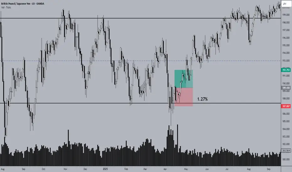
Market Condition, Trading Conditions and StrategiesHere are some important terms for traders to understand.
Market Condition refers to the overall long-term trend, where we are in the CYCLE of the Stock Market.
Trading Conditions are identified and traded by using the day over day and week over week trends and trendline patterns within that Cycle.
Strategies relate to a specific trading style based on the current Market Condition and the Trading Condition(s) within that particular Market Condition.
The Market is in a Moderately Uptrending Market Condition at this time. Trading conditions vary from sideways trends to Velocity runs, to minor corrections.
The market is choppy and sideways. Volatile markets have huge white and black candles that change abruptly from one day to the next based upon WHO IS CONTROLLING price.
In the sideways trend we’re experiencing now, different market participants are taking different actions:
Professional Traders are mostly trading to the upside.
There are also smaller funds managers with less than $3 billion in assets under management, aka Retail Side Asset Managers.
There are fewer retail investors and retail traders are mostly sidelined right now since they are worried.
There is some minor Dark Pool rotation to lower inventories of specific stocks in the NASDAQ 100 index, which impacts the QQQ ETF.
Understanding the dynamics of the Stock Market helps you trade with confidence, making decisions based on real market conditions instead of retail news—which is always late and often drives manipulative activity.

When Crypto Actually MovesCrypto trades around the clock, but the market doesn’t behave the same way at every hour. Volume, liquidity, and volatility cluster around predictable windows, and those windows shape how setups form and how price reacts. When you understand these shifts, you stop taking trades randomly and start aligning execution with the moments when the market truly moves.
Why Sessions Matter
Even though crypto never sleeps, human traders and institutional desks still operate in cycles. Liquidity providers adjust during business hours. Market makers re-balance at session opens. Macro news is released on a fixed schedule. These patterns create recurring volatility signatures.
Ignoring sessions means you treat every candle as equal. Understanding sessions means you add a layer of context that improves timing, risk control, and win rate.
Asia Session (00:00–06:00 UTC)
The Asia window tends to be slower and more range-bound.
Characteristics include:
– Moderate liquidity
– Clean consolidations
– Accumulation before Europe
– Fewer impulsive moves unless driven by news from Asia-Pacific regions
This period often sets the initial range of the day. Liquidity begins to cluster above highs and below lows, creating the conditions for later sweeps.
Europe Session (07:00–12:00 UTC)
Liquidity expands significantly as London opens. You often see the first engineered move of the day.
Key behaviors:
– Early sweeps of the Asia range
– Strong breakouts from overnight compression
– Directional push before New York volatility
This session frequently defines the directional bias into US hours. It’s a prime window for structured setups because market participation rises sharply.
US Session (13:00–20:00 UTC)
This is the most active window. The highest liquidity and most decisive moves occur here.
Typical features:
– Strong continuation or full reversal of the London move
– Reaction to economic news
– Trend acceleration during peak overlap hours
This is where major breakouts, deep liquidity hunts, and high-powered moves happen. If you trade momentum or breakout strategies, this session offers the cleanest conditions.
Weekend Behavior
Weekends operate on thin liquidity. Order books are lighter, market makers are less active, and volatility behaves differently.
Common outcomes:
– Sharp wicks that violate structure
– Sudden spikes without follow-through
– False breakouts with immediate reversals
Weekend moves often distort technicals. They can be useful for narrative-driven positions but carry higher risk for intraday traders.
How to Integrate Sessions Into Your Trading
Use sessions to filter when you participate and when you avoid noise.
Practical adjustments:
– Execute momentum setups during Europe or US hours.
– Treat Asia session as a range-building phase suitable for scouting zones.
– Avoid taking aggressive positions during weekend chop.
– Use session opens as key decision points for liquidity grabs.
When you layer session timing on top of structure, you refine entries and eliminate trades that lack the environment for follow-through.
The Strategic Advantage of Session Awareness
Session timing gives you clarity. You start anticipating where liquidity is likely to be engineered, where volume will enter, and when the market is likely to trend or stall.
This transforms your approach.
Instead of reacting to candles, you plan around expected volatility cycles.
Instead of forcing trades, you wait for session transitions that historically produce reliable movement.

Liquidity Basics: Equal Highs/Lows, Inefficiencies & POIsPrice doesn’t move randomly, it is always attracted towards liquidity.
Every wick, breakout, and fake-out tells a story of orders being filled.
If you can read where those orders are hiding, you stop trading noise and start trading intention.
Equal Highs & Lows — The Obvious Targets
Retail traders love to mark equal highs and lows as “strong support/resistance.”
Smart money sees them as fuel.
Above equal highs = cluster of buy stops.
Below equal lows = cluster of sell stops.
When price reaches them, it’s a collection of accumulated liquidity as a main driver behind that move.
Inefficiencies — Fair Value Gaps
Also known as Fair Value Gaps (FVGs) or imbalances, these occur when price moves too quickly, leaving unfilled orders behind.
Price often revisits these zones later to rebalance.
Spot them between large candles with no overlap, they often mark where institutions filled partial orders.
Points of Interest (POIs)
POIs are areas where liquidity and inefficiency converge , the zones of intent.
Look for:
Liquidity sweep of equal highs/lows
Return to imbalance or order block
Shift in market structure
That’s where high-probability setups occur.
Note:
Stop chasing every candle.
Start mapping why price moves.
Equal highs and inefficiencies are magnets, with proper plan and confluence this can represent your strong side of trading.

A High-Impact Support Zone Meets a Breakout StructureIntroduction
Markets occasionally compress into areas where structure, momentum, and historical buying pressure align with surprising precision. When that compression occurs at a major higher-timeframe floor, traders often pay closer attention—not because the future is predictable, but because the chart reveals a location where price behavior typically becomes informative.
The current case study centers on a market pressing into a high-impact support zone visible on the monthly chart, while the daily chart displays a falling wedge pattern that has gradually narrowed the range of movement. This combination often highlights moments where the auction process is nearing a decision point. The purpose here is to dissect that confluence using multi-timeframe structure, pattern logic, and broad order-flow principles—strictly for educational exploration.
Higher-Timeframe Structure (Monthly)
The monthly chart shows price approaching a well-defined support area between 0.0065425 and 0.0063330, a region that has acted in the past as a base for significant reactions. These areas often develop because markets rarely absorb all buy interest in a single pass; pockets of unfilled orders may remain, leading to renewed reactions when price returns.
This type of zone does not guarantee a reversal. However, historically, when price reaches such levels, traders tend to monitor whether selling pressure slows or becomes less efficient. In this case, the structure suggests a recurring willingness from buyers to engage at these prices, forming a foundation that has held multiple swings.
The presence of a clear, higher-frame resistance at 0.0067530 anchors the broader range. When price rotates between such boundaries, the monthly context often acts as a roadmap: major support below, major resistance above, and room in between for tactical case-study exploration.
Lower-Timeframe Structure (Daily)
Shifting to the daily chart, price action has carved a falling wedge, a pattern often associated with decelerating downside movement. In wedges, sellers continue to push price lower, but with diminishing strength, as each successive low becomes less effective.
This type of compression structure can provide early evidence that the auction is maturing. Traders studying such patterns often watch for:
tightening of the range,
shorter waves into new lows,
initial signs that buyers are defending intraday attempts to drive price lower.
The daily wedge in this case sits directly on top of the monthly support zone—an alignment that strengthens its analytical relevance. The upper boundary of the wedge sits near 0.0065030, and a break above that line is often interpreted as price escaping the compression phase.
Multi-Timeframe Confluence
Multi-timeframe confluence arises when higher-frame structure provides the background bias and lower-frame patterns offer the tactical trigger. In this case:
The monthly chart signals a historically responsive support zone.
The daily chart shows structural compression and slowing downside momentum.
The interaction between them creates a scenario where educational case studies tend to focus on breakout behavior, as the daily timeframe may provide the first evidence that higher-frame buyers are engaging.
This confluence does not imply certainty. It simply highlights a location where structure tends to become more informative, and where traders often study the transition from absorption to response.
Order-Flow Logic (Non-Tool-Specific)
From an order-flow perspective, strong support zones typically develop where prior buying activity left behind unfilled interest. When price returns to that region, two things often happen:
Sellers begin to encounter difficulty driving price lower, as remaining buy orders absorb their activity.
Compression patterns form, as the market oscillates in a tightening range while participants test whether enough liquidity remains to cause a directional shift.
A breakout of the daily wedge represents a potential change in the auction dynamic. While sellers are still active inside the wedge, a breakout suggests their pressure may have become insufficient to continue the sequence of lower highs and lower lows. Traders studying market transitions often use such moments as part of hypothetical scenarios to understand how imbalances evolve.
Forward-Looking Trade Idea (Illustrative Only)
For educational purposes, here is how a structured case study could frame a potential opportunity using the discussed charts:
Entry: A hypothetical entry could be placed above the falling wedge, around 0.0065030, once buyers demonstrate the ability to break outside the compression structure.
Stop-Loss: A logical invalidation area in this case study would be at or below the monthly support, around 0.0063330, where failure would indicate the higher-timeframe zone did not hold.
Target: A purely structural wedge projection would suggest a target near 0.0067695, aligning closely with the broader resistance region on the monthly chart.
These price points yield a reward-to-risk profile that is measurable and logically linked to structure, though not guaranteed. This case study exists solely to illustrate how support-resistance relationships and pattern logic can be combined into a coherent, rules-based plan, not as an actionable idea for trading.
Yen Futures Contract Context
The larger (6J) and micro-sized (MJY) versions of this futures market follow the same underlying price but differ in exposure and margin scale. The standard contract generally carries a greater notional value and therefore translates each price movement into a larger monetary change. The micro contract mirrors the same structure at a reduced size, allowing traders to adjust position scaling more precisely when navigating major zones or breakout structures such as the one discussed in this case study:
6J equals 12,500,000 Japanese Yen per contract, making it suitable for larger, institutional players. (1 Tick = 0.0000005 per JPY increment = $6.25. Required Margin = $2,800)
MJY equals 1,250,000 Japanese Yen per contract, making it suitable for larger, institutional players. (1 Tick = 0.000001 per JPY increment = $1.25. Required Margin = $280)
Understanding margin requirements is essential—these products are leveraged instruments, and small price changes can result in large percentage gains or losses.
Risk Management Considerations
Strong support zones can attract interest, but risk management remains the foundation of any structured approach. Traders studying these transitions typically:
size positions relative to the distance between entry and invalidation,
maintain clear exit criteria when structure fails,
avoid adjusting stops unless the market has invalidated the original reasons for the plan,
adapt to new information without anchoring to prior expectations.
These principles emphasize the importance of accepting uncertainty. Even at major support zones, markets can remain volatile, and scenarios may unfold differently than anticipated.
When charting futures, the data provided could be delayed. Traders working with the ticker symbols discussed in this idea may prefer to use CME Group real-time data plan on TradingView: www.tradingview.com - This consideration is particularly important for shorter-term traders, whereas it may be less critical for those focused on longer-term trading strategies.
General Disclaimer:
The trade ideas presented herein are solely for illustrative purposes forming a part of a case study intended to demonstrate key principles in risk management within the context of the specific market scenarios discussed. These ideas are not to be interpreted as investment recommendations or financial advice. They do not endorse or promote any specific trading strategies, financial products, or services. The information provided is based on data believed to be reliable; however, its accuracy or completeness cannot be guaranteed. Trading in financial markets involves risks, including the potential loss of principal. Each individual should conduct their own research and consult with professional financial advisors before making any investment decisions. The author or publisher of this content bears no responsibility for any actions taken based on the information provided or for any resultant financial or other losses.
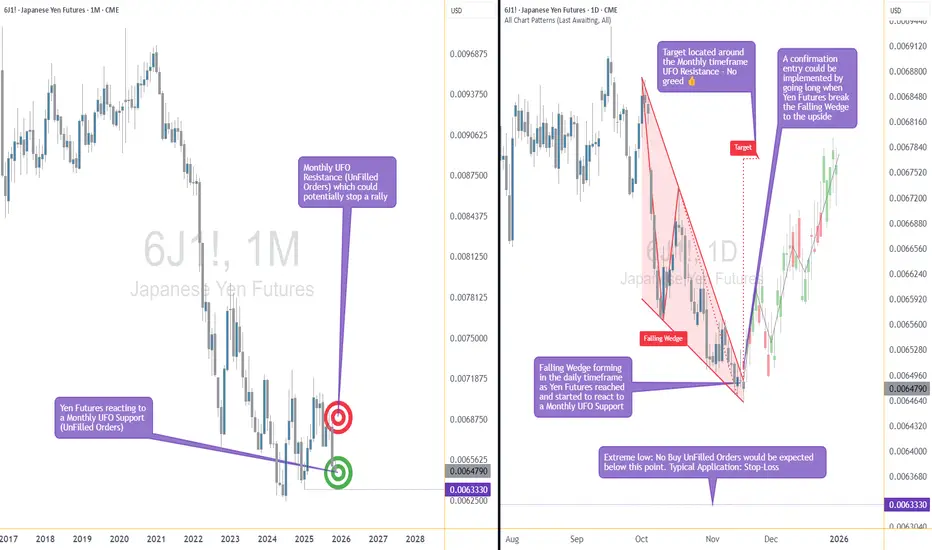
Price moves in a very specific way...In this short video I go through a bit of lower timeframe price action on the ETH futures chart.
Yeah, it is pretty straight forward and is just another example of price moving in terms of liquidity, efficiency, and fair value on a fractal nature.
R2F Trading

Bitcoin: What Historical Drawdown in a Bear Market?Since its all-time high at $126,000 reached on October 6, Bitcoin has been following a series of corrective sessions. This pullback raises a key question: is it merely a consolidation within a bull market, or the beginning of a true bear market?
First, if the cycle really ended on Monday, October 6, this would still align with the classic 4-year timing cycle, with a duration that fits within the multi-criteria average (see my correspondence table below) of previous cycles.
At this stage, the downtrend is not confirmed, as key supports — notably the weekly Ichimoku cloud — have not been broken. This level marks the decisive boundary between a standard cycle correction and a deeper reversal.
As long as the price remains above the Kumo, the bull cycle that began in 2022 remains structurally valid. Historically, Bitcoin only enters a bear market when weekly candles close below the cloud, along with the chikou also falling below price. Such a configuration would signal a durable deterioration in momentum for the coming months.
If this zone were to give way, then shifting to a full bear-market framework would become relevant. To estimate a potential bottom, the most useful tool remains the drawdown indicator from ATHs, which measures the percentage decline from the previous all-time high. The chart clearly shows a long-term trend: drawdown bottoms form along a rising diagonal since 2011, while the intensity of declines gradually decreases cycle after cycle.
Historical numbers confirm this:
• 2011: –93%
• 2015: –86%
• 2018: –84%
• 2022: –77%
This gradual reduction reflects market maturation and increasing market capitalization. Extrapolating this trend places the theoretical next trough between –70% and –76%. This is also the zone highlighted on the chart as long-term historical support.
Applying these percentages to the $126,000 peak yields:
• –50% → $63,000
• –65% → $45,000
• –70% → $37,800
• –73% → $34,000
• –76% → $30,200
These levels therefore form a probable bottom range in the still-unconfirmed scenario of a bear market. They also correspond to major technical zones frequently observed at cycle junctions.
Finally, the average duration of Bitcoin bear markets — traditionally around 12 months — suggests a theoretical bottom around late 2026, if the October 2025 top were indeed a cycle peak.
In summary:
We are not in a bear market as long as major technical supports hold. The market is now clearly at a technical crossroads. But if a breakdown occurs, historical drawdown patterns suggest a statistical bottom between $40,000 and $60,000, within a timeframe of roughly one year.
DISCLAIMER:
This content is intended for individuals who are familiar with financial markets and instruments and is for information purposes only. The presented idea (including market commentary, market data and observations) is not a work product of any research department of Swissquote or its affiliates. This material is intended to highlight market action and does not constitute investment, legal or tax advice. If you are a retail investor or lack experience in trading complex financial products, it is advisable to seek professional advice from licensed advisor before making any financial decisions.
This content is not intended to manipulate the market or encourage any specific financial behavior.
Swissquote makes no representation or warranty as to the quality, completeness, accuracy, comprehensiveness or non-infringement of such content. The views expressed are those of the consultant and are provided for educational purposes only. Any information provided relating to a product or market should not be construed as recommending an investment strategy or transaction. Past performance is not a guarantee of future results.
Swissquote and its employees and representatives shall in no event be held liable for any damages or losses arising directly or indirectly from decisions made on the basis of this content.
The use of any third-party brands or trademarks is for information only and does not imply endorsement by Swissquote, or that the trademark owner has authorised Swissquote to promote its products or services.
Swissquote is the marketing brand for the activities of Swissquote Bank Ltd (Switzerland) regulated by FINMA, Swissquote Capital Markets Limited regulated by CySEC (Cyprus), Swissquote Bank Europe SA (Luxembourg) regulated by the CSSF, Swissquote Ltd (UK) regulated by the FCA, Swissquote Financial Services (Malta) Ltd regulated by the Malta Financial Services Authority, Swissquote MEA Ltd. (UAE) regulated by the Dubai Financial Services Authority, Swissquote Pte Ltd (Singapore) regulated by the Monetary Authority of Singapore, Swissquote Asia Limited (Hong Kong) licensed by the Hong Kong Securities and Futures Commission (SFC) and Swissquote South Africa (Pty) Ltd supervised by the FSCA.
Products and services of Swissquote are only intended for those permitted to receive them under local law.
All investments carry a degree of risk. The risk of loss in trading or holding financial instruments can be substantial. The value of financial instruments, including but not limited to stocks, bonds, cryptocurrencies, and other assets, can fluctuate both upwards and downwards. There is a significant risk of financial loss when buying, selling, holding, staking, or investing in these instruments. SQBE makes no recommendations regarding any specific investment, transaction, or the use of any particular investment strategy.
CFDs are complex instruments and come with a high risk of losing money rapidly due to leverage. The vast majority of retail client accounts suffer capital losses when trading in CFDs. You should consider whether you understand how CFDs work and whether you can afford to take the high risk of losing your money.
Digital Assets are unregulated in most countries and consumer protection rules may not apply. As highly volatile speculative investments, Digital Assets are not suitable for investors without a high-risk tolerance. Make sure you understand each Digital Asset before you trade.
Cryptocurrencies are not considered legal tender in some jurisdictions and are subject to regulatory uncertainties.
The use of Internet-based systems can involve high risks, including, but not limited to, fraud, cyber-attacks, network and communication failures, as well as identity theft and phishing attacks related to crypto-assets.
